Research

Deployment-Ready RL: Pitfalls, Lessons, and Best Practices
This text is a transcript of a webinar led by Kyle Morgenstein from the University of Texas at Austin for the Humanoid team. We’re sharing it on our blog to spread knowledge and help move the humanoid robotics industry forward. Please note that the views and information presented here are Kyle’s own.
Kyle Morgenstein, University of Texas at Austin
02:59 –> 03:38
As much as I’d like to sit here and give a lecture on proximal policy optimization and math, that’s not the goal today. Today we want to be pretty laser-focused on deployment on what does it mean to take our policies from simulation and get them to work on hardware.
03:38 –> 04:38
In the last couple of years, we’ve seen this really incredible success in legged locomotion, specifically in quadrupeds, using reinforcement learning.
Compared to model-based methods in the years prior we’re now able to do things that we thought were impossible. Learning entirely in simulation and deploying in the real world. So here we see some of the vision-based RL parkour work coming out of ETH Zurich, uh, without any kind of references or contact schedule, or any of the things that would have been required in model-based control.
We can put these robots sort of anywhere on Earth, and they’ll navigate them very effectively.
And then maybe my favorite video that’s come out in recent years has been this ladder climbing video. When I first saw it, I couldn’t believe what I was seeing. And of course, there are some modifications to make this problem a little bit easier. There’s the foot design that has the hook.
But the fact that we’re able to learn these really, really complex and agile skills in simulation and then deploy them in the real world, zero-shot is, I think, incredibly impressive.
04:38 –> 05:38
And we’ve seen this work as a standardized recipe now that works on any quadruped you can imagine.
When seeing these sorts of results over the last couple of years, I think there’s a fairly natural question that arises. Which is why we haven’t seen the same degree of success in humanoids?
So I want to show a video from last year. It was a humanoid parkour paper copying some of the best practices that came out of those ETH parkour papers. And to be clear, this is an incredibly impressive result as well. The vision-based policy adapting to its environment. Taking large steps, jumping over gaps. It’s still a very, very good policy, but the robot exhibits an ailment that we call “Drunken Robot Syndrome”. The gait is not quite confident. It’s taking all these small stutter steps to orient itself.
05:38 –> 06:38
And maybe this makes sense in simulation, given that our largest penalty that we ever give it is a termination for falling over, so the robot learns that it needs to stay upright at all costs, it’s taking these small steps to reorient itself.
There’s sort of an old adage that you don’t have to worry about dynamic balance if you can just step fast. And so we see this good enough transfer of a lot of these ideas that have worked so well in quadrupeds, but we don’t quite see the same level of precision and smoothness that we see in quadrupeds transfer over into humanoids. And so I’d like to spend some time today talking about what are those gaps in the deployment side that take us from the kinds of precise, agile policies we see in simulation, and turn them into behaviors on the robot.
To act as a foil for this, and maybe to contradict everything I just said, has been this demo from earlier this year where Boston Dynamics Electric Atlas did these really, really slick and smooth walking and running and dancing behaviors.
I think that there’s a pretty clear distinction between the video on the left and the right.
06:38 –> 07:38
The video on the left, the humanoid parkour, is using sort of the vanilla RL formalism. We’ve got our rewards, we hand-design, we hand-tune them, and we get the behavior that we want. On the right, these really nice behaviors are coming from reference data. So we have some motion capture data and retarget it for the robot, in this case, just kinematic retargeting, and then we can embed that in the RL formalism to get these kinds of really, really smooth behaviors.
And so I think that there’s sort of a conflict or tension between what we can do to take our vanilla RL formalism that works so well in the quadruped case, in the quadruped case we don’t require any additional references at all. Versus in the humanoid case, where we’d like to see the same kind of vanilla RL formalism work, but we haven’t really seen that at a deployment level.
And we’re starting to see a lot more of these reference and imitation methods embedded into RL to try and get that same degree of performance. That’s the starting point for what I want to talk about today.
07:38 –> 09:38
To that end I want to talk about actions-based design, the observation space, how you deal with model mismatch, things like your actor, your student-teacher, actor-critic methods, or asymmetric actor-critic. Some basic intuition for reward tuning, and then finish up with some talk about RL with motion references, and maybe how the field is evolving around it.
And you can see, I come from more of a control theory background, but have now turned my PhD into a learning PhD. And I’m strongly of the belief that to be able to do this well, you do need a very strong mix of learning and control theory. The intuition that you get from control theory is really indispensable. But the methods from learning are really what has enabled us to deploy these policies on even low-quality hardware very, very robustly. So, with that, let’s jump into it.
Starting with the action space. Typically, the action space that we use for these policies is a joint position residual.
08:38 –> 09:38
And so that looks like our PD control law at the top, so we have some desired joint position Q, and some velocity Q dot, and we track it. Now we take our action, we sample from our policy, parameterized by our weights. And our desired position, we say, is some reference position, maybe it’s the stance configuration for our robot, plus the scaled output from our neural network. And our desired velocity is always zero, so it’s gonna act like a regularizer for us.
This gives us our fairly standard control law. It’s still a PD control law, where we have some residual on top of a stance position, and that’s giving us the behavior that we want. This is sort of a virtual spring, it’s a damped virtual spring. It’s one way of thinking about it. But I’d like to convince you that there’s an alternative way of thinking about this that makes it a lot easier to deploy.
So, if you algebraically rearrange, if you pull the KAA term outside of the stiffness term, then you can treat this equivalently as a joint position residual.
09:43 –> 10:38
Or as a feed-forward torque with gravity compensation. And there’s the dimensions on the neural network output A don’t really care either way, but the way you look at these equations makes a big, big difference in how you tune them. Specifically when you go to tune the PD gains and the action scale A.
Given these two different representations of our action, we’d like to try and determine a pretty robust way of selecting our gains, both that we get good exploration in simulation, as well as good deployment on our hardware.
So the two terms we have are gravity compensation, as opposed to our feed-forward torque.
10:38 –> 11:38
Now, notice that even though these are algebraically equivalent lines, this is actually a multi-rate loop, so the Kp term, or the PD term, the first term in the bottom equation, is being updated at your firmware rate, so that could be somewhere in the thousands to tens of thousands of hertz.
Whereas the feed-forward torque term is only being updated at the policy control rate, which is usually around 50 Hz. Similarly, the joint position residual version of this. The whole control law is being updated at that firmware rate, but you’re only updating the action at that 50Hz.
What that means is that from the perspective of the PD controller, the action is quasi-static. It’s effectively not moving. If you’re updating your PD controller at 40,000 Hz, and your action only updates at 50. That’s more or less a static action for the PD controller to track.
So you can think of this either as a gain-tuning problem in the physical sense…
11:38 –> 12:38
…where we’d like to find a KP and KD such that we can converge on the position offset given to us by KA times A, and track that high rate, high fidelity to be able to achieve the desired position residual by the time we get our next control input.
Alternatively, we can think of this as adding some constant feed-forward torque onto this high-rate PD control law that’s smoothing out jitter or other disturbances from the policy. The difference that this makes is how you pick your gains, so you can either choose to… if you treat this as a PD controller in the typical control sense, then you’re gonna pick KP to be the square of your natural frequency, and use that KD to be critical damping and things like that. And the resulting gains are very, very high.
And so that will transfer to hardware, you’ll be able to stand the robot up no problem, because you’re treating it as a sort of physical problem. But you have substantially reduced exploration performance in simulation.
12:38 –> 13:38
If your gains are very, very high, then the effective bandwidth of the policy learn is lower, I’ll show that visually in a moment. But in the low gains case, where you’re in the bottom equation, where you’ve got your gravity compensation you’re allowing the policy to determine the bulk behavior, and you’re just using the PD controller as a bias towards stance.
So as opposed to treating the action as a position, you have to track exactly. You can treat the PD controller as just sort of a nudge at the beginning of training to keep you oriented around stance and to smooth out any jitter, and then the policy gets to learn the whole behavior around that.
So to depict this visually, let’s assume that at the beginning of training, our neural network is parameterized as a Bolivariate Gaussian, let’s call it one-dimensional for now. So its shape is gonna look like this black curve. So this is our distribution of actions that we may sample at the beginning of training.

Given some torque limit for our robot, we’d like to be able to understand what kind of exploration we can perform at the beginning of training.
13:38 –> 14:38
In the high-gain case, it’s going to be the red dotted lines. Because of our torque limits and our gains being as high as they are, when you do your random sampling over your untrained policy, the bandwidth, the range of values that you can sample, where you change the position of the actuator, or where you have a difference in output torque before it gets clipped, is very, very small.
It means that even though you’d like to sample from this normal distribution centered at zero, you end up oversampling and biasing your exploration at the torque limits. Because the high stiffness means that it’s effectively a bang-bang controller. So you’re exploring moving your joint one direction, you’re exploring moving it the other direction, but it’s hard to sample in between because there’s a very limited bandwidth that you’re able to resolve before you hit those torque limits when your gains are high.
When you have the lower gains, you’re able to resolve a much larger range of the distribution that you’re sampling from, this full normal curve.
14:38 –> 15:38
And so this gives you much, much better exploration, because now, let’s say if I want to sample on the right side of the distribution, and I’m over here close to but under the dashed blue line.
And then as opposed to that sample, let’s say half of that, but it’s still outside of the red dotted lines. That difference, when I’ve got low gains, I can track. The policy will take a different behavior, it’ll get to a different joint position. And we’ll get different rewards for it, we got good learning signal, we’ll update accordingly.
In the high gains case, in either one of those samples, I’m still gonna hit my torque limit, and so the joint’s still going to its maximum value. And so, you end up with a very jittery policy that is hard to do exploration with, and oftentimes won’t converge.
And so when you have lower gains, you tend to get much, much better training performance, uh, you end up with a smoother policy, it sort of helps the whole problem, not because it’s of the physical system.
If we go back to the equation for a minute. It’s not that, you know, one of these equations is more correct than the other, they’re both true.
15:38 –> 16:38
But if you think about it as a feed-forward torque law, as opposed to a joint position residual, it’s much, much easier to tune these parameters for exploration and simulation.
It’s not necessary to tune them as if it were a physical system that you must track as a standard PD control law, or you want to minimize overshoot and rise time and everything else like that. We don’t have to think about it in that control theoretic sense.
It’s better to think about it as an inductive bias against stance early in training. Really, what the action scale Ka is doing for you is – it’s controlling your learning rate, or your sampling rate, your exploration rate. So in Ka is very high, you’re going to oversample the torque limits.
But you’re going to more rapidly explore that space, whereas when Ka is low, you’ve got maybe lower magnitude exploration, so it can take longer to get momentum and energy in the weights of the neural network to output large values. But you get much smoother policies as a result.
17:38 –> 18:38
Just last thing to say on this visual, which is that when you have the high-gain case, you have limited bandwidth, like I mentioned, because you’re effectively doing bang-bang control. Uh, the effect of this when you’re training is that your actor standard deviation may increase, and in my opinion, this is sort of the most critical parameter to track during training, more than your terminations, more than your rewards, more than your success metrics.
If your standard deviation does not converge, then all of your training is sort of kaput. You’re not going to be able to reason about the effects of the policy with an increasing standard deviation, and I’ll talk more about that in depth in a little bit.
But that’s one of the big risks here, is if you have the high gains, even though it may be easier to start training, because you start with more torque at your stance configuration, the risk to the learning rate, the risk to the exploration is such that it’s generally not worth it. You generally do want the lower gains here.
I will talk about what that means on hardware in a minute. Um, but then, how do you pick those gains, heuristically?
This is sort of where we’re leaving well-principled theory land, and now going into what works in practice.
18:38 –> 19:38
This is just a heuristic. But the way I like to think about it is, given some range of motion at the joint and given some torque limit, we set Kp such that when we’re at one extreme of that range of motion, you can’t apply more than your torque limit. So this helps protect the system mechanically as well.
You can also modify this so that your spring is defined with respect to the center point. If you assume that you’ve got a symmetric range of motion. But I tend to find that it works better if you just treat it as… let’s say I’m at one extreme of my range of motion and I’d like to get to the opposite extreme of my range of motion. I set my Kp such that I would exhort maximum torque to cross over from one extreme to the other.
I think this works quite nicely in practice, because we very, very rarely, in a single step, want to transition from one extreme to the other. And so we’re generally using much less than this torque limit but we give the controller authority up to that torque limit to actuate the joint.
19:38 –> 20:50
But we don’t risk exceeding that. And then to set the damping for this. Again, just a heuristic, if you divide Kp by about 20, I find that works really nicely in practice.
25:38–> 26:43
Right, so then given this heuristic, I think there’s a fair question, especially that I typically get from the roboticists and mechanical engineers of how do I actually deploy a low-gain policy, because how am I tracking my joints otherwise?
So, a couple different ways to do it. First is a robot that we have in my lab, Spot, which we use for RL quite a bit. If you have high fidelity, torque or current feedback, and especially if you have output torque sensing, it is very, very easy to deploy a low-gain policy, because that feed-forward torque term can be tracked by your low-level control.
If you have that, that really makes life very easy. Spot is by far the easiest robot I’ve ever done RL with, because it has output torque sensing. And so that means that whatever, you know, torque I ask for, it’s gonna give me.
Like I mentioned, you can also anneal the gains to zero. As opposed to having to set a control law with low gains into your firmware, your low-level controller, you can just send a desired torque and If you have good enough torque tracking, that will work.
26:43–> 27:38
Although you do end up a little bit more susceptible to modeling errors, because you don’t have that PD controller to smooth out jitter from things like unmodeled joint friction or roadrunner show.
You can also train an actuator network if you have some reference policy to collect data with, like a model-based policy. That works quite well.
Or you can just distill it into a high-gain policy. So maybe you’re working with your physical system, and with low gains, you just can’t get it to track the torque accurately enough.
The reason we use low torques in sim is primarily for exploration. It gives us better exploration characteristics early in training, so we can learn more agile and more precise behaviors.
Once you have a policy that can provide you those references, you can then distill that with a student-teacher method into a policy that uses the higher gains that do work on your hardware, and then just track the desired joint positions accordingly.
27:38–> 28:38
And so there is some flexibility. What you train in simulation, it doesn’t always have to mirror exactly what you deploy on hardware, and we’ll talk more about some of those methods for distillation in a little bit.
Now let’s talk about the observation space.
I very, very often see people throwing wild things into their observation space that do not need to be there. All you need for your observation space are your velocity, your orientation, your joint state, your last action, and your command. That’s it.
You do not need anything else, you do not need a time history. If you need anything besides these features, you have to have a good reason for it. The one-time step should be all you need.
28:38–> 29:38
Even when you’re doing perceptive RL, then you can add and ensure a height scan or a depth image. Your command term, you can have multiple different types of commands. Velocity tracking is the common one, but this could also be a desired position and navigation, or a desired base height, or a desired footstep frequency, so that the command can still be somewhat expressive.
But in terms of the representation of the robot’s state. This is all you need. And for orientation, projected gravity is a much easier space to learn in than quaternions. I would recommend using projected gravity here as well.
The one exception, or a couple exceptions, are if you have a good reason for it. Some good reasons may be motion imitation. If you’re trying to learn some trajectory that you’ve already recorded, maybe through motion capture, then it’s reasonable to observe references for that trajectory that the policy is trying to meet, so that they’re joint targets at that point.
Or to observe the phase of the motion.
29:38–> 30:38
Similarly, in navigation, what made a lot of the animal navigation and parkour papers work through RSL was observing a clock that was counting down how much time remained in the episode, and this is really helpful to teach the policy that it didn’t need to throw its body into the goal region.
They could walk there much more steadily, because it knew it had time left before it was going to be reset.
Similarly for local manipulation, maybe you’d like to observe some objects or forces or goal positions for those objects. These are all good reasons to augment the observation space. But when you go to augment it, you do need to have a good reason for it.
Anything else is generally an excuse for poor system identification, so I see people add in things like the estimated ground friction. You don’t need that. Or estimating the desired foot height, you don’t need that.
Uh, in general, if you’ve got a well-identified system, you do not need anything additional to your observation space. So I’ll give an example of this. It’s sort of a cardinal sin I see in papers all the time related to linear velocity.
30:38–> 31:38
Uh, typically, especially for the… a lot of the Unitree robots, they don’t have a very good linear velocity estimator on the robot. So, there’s a couple different ways you can do this estimation. Of course, the more traditional way is just to use a model-based estimator, a common filter, a factor graph, etc. It might take a week or two to write out and test, and that’s fine, but it does help you substantially. If your goal is velocity tracking, it’s pretty important to know what your velocity is.
But there are alternatives, it doesn’t have to be a Kalman filter. So, for example, the paper on the diagram on the right is a learned velocity estimator. It’s a concurrent training, it’s a paper out of KAIST, very nice paper. This is very easy to implement. You could implement this in Isaac Lab in maybe an afternoon, train it at about the same time.
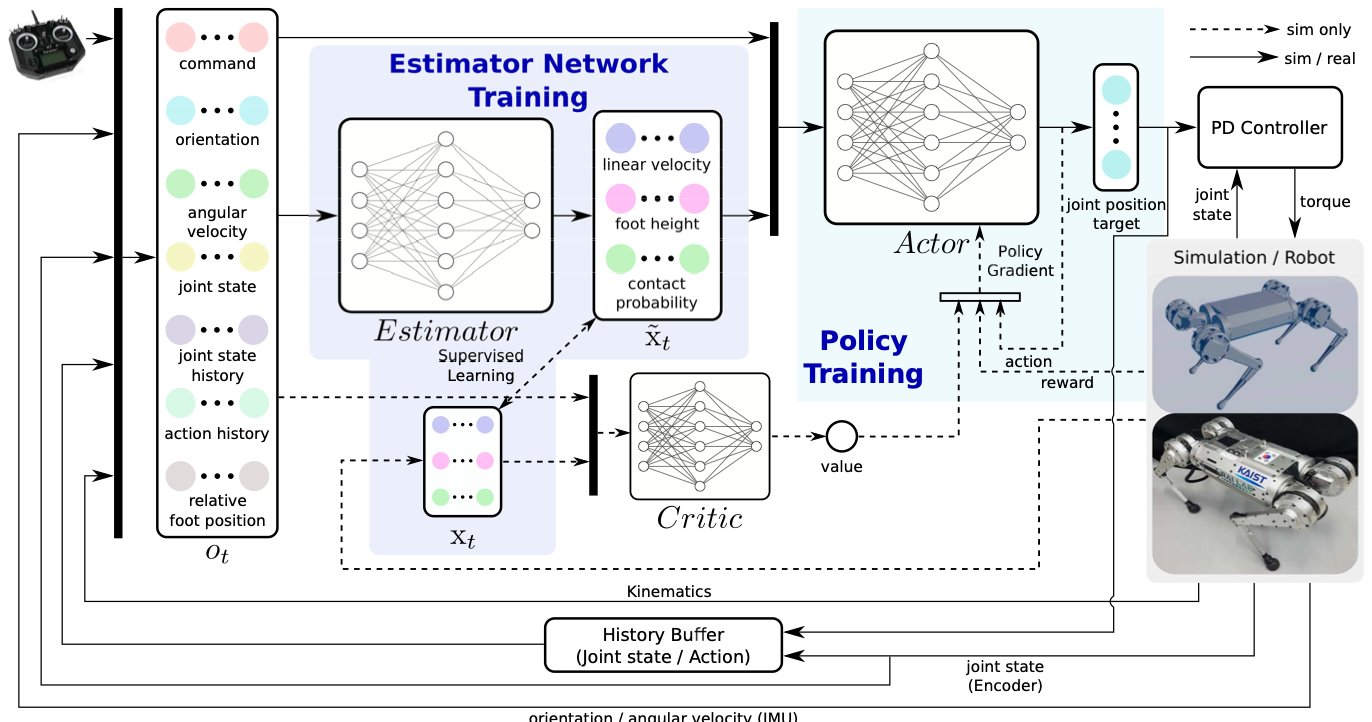
Ji et al., KAIST
And this Learn module will give you an estimate of the linear velocity and foot height and contact state for the feet, and that’s all really helpful information to have. If you have that information available to you, that’s fine, you can use it.
31:38–> 32:38
But you should estimate it in some way. And then you can also do implicit estimation, so it’s become pretty common to use decoding heads, which we’ll talk more about in a little bit. But in some way, you should be embedding the linear velocity into your policy.
What you should not be doing is augmenting the observation space and hoping that it works. That’s what most people do. So, as opposed to having any kind of explicit or implicit estimate of the linear velocity, they’ll typically just add on an observation history. And say, okay, well, you know, I have all of my positions. And if I have enough time steps, then through finite differencing, the policy should just figure out how to reason about the velocity terms.
And it may, but this is less effective than using explicit estimation basically every single time.
Similarly, for recurrent architectures, there are reasons to use those architectures. We’ll talk about it in a minute. But lack of state estimation is not a good reason. If you have the ability and bandwidth to give yourself an estimate, you will be much, much happier. You will spend more time tuning the right things in your control policy.
32:38–> 33:38
You’ll have more time to spend with your spouse and kids. You’ll be a happier person, you’ll have lower stress. If you have the ability to train a state estimator, or use a model-based estimator, you should do it. It really, really, really helps.
I see it so often, these really complex architectures and papers that could all be resolved if they just had a state estimator. Model-based control will set you free. It does work.
There are times when it is okay to augment the observation space, or to violate Markov property, though the sort of context for everything we’re doing here in RL is as a Markov decision process, where we assume that one time step is sufficient to define your full problem space, but there are exceptions.
For example, maybe your task is acceleration-dependent, and you don’t observe your accelerations directly. So maybe you’re doing force control, and you don’t have IMUs on your end effectors.
Then you can use some amount of observation history or recurrent architecture, all the things I just said not to do, but when your task requires it, that’s okay.
33:38–> 34:38
You’re not making this assumption that you need it. It is true that through finite differencing, you can approximate these acceleration terms, and if your rewards are acceleration-dependent as well, then the policy will learn to reason about it.
Similarly, if your task requires memory, so if you’re trying to navigate a maze, then knowing that you took the left last time, and now you’d like to take the right, that’s pretty helpful. You do need to know that in your observation in some space.
Uh, so usually people do this by using a memory module, like neurovolumetric memory or some other technique like that, or using an explicit representation of your environment, like an occupancy map.
And so if you have access to this information, that will substantially help your training performance. But again, the idea is don’t just naively throw recurrent architectures or histories at the problem. I think the original RMA paper used 50 time steps. You do not need one second of history in 99% of cases. It’s usually overkill, and it usually just hurts your training performance.
34:38–> 35:38
Then the last one is when there’s some kind of fundamental constraint. So maybe you’ve got some non-rigid contacts that one time step is not enough to reason about how the trampoline may respond to your behavior, or you’ve got very, very poor quality sensors that you can’t extract the information you want.
If it’s possible, just fix the fundamental limitation, that will always help you more. Most of the struggle of RL is not actually a problem with learning, it’s the hardware, it’s the engineering, it’s the tooling, it’s everything around the RL. So, fix that first. It’ll make the learning problem much, much easier.
But if you’ve tried all of these things, and it’s still not working the way you expect, you can find better performance with these sorts of histories, but usually at the cost of conservatism in the policy.
35:38–> 36:38
Now I want to spend a little bit of time dealing with model mismatch.
Usually, like I mentioned, we’re treating this as a Markov decision process, but it’s specifically a partially observable Markov decision process, and so depending on where that partial observability comes from, we may need to change something fundamental about our learning architecture, oral neural network architecture that makes the problem tractable.
And so one example of this may be where you have informationally dense data type on your hardware, something like an image, but that doesn’t provide you an explicit representation of state, going back to control theory formalisms.
So, in your simulator, you have privileged information, ground truth, everything you could ever want about the position of your feet and the position of objects around you and everything else like that. But on your real robot, maybe you don’t have a depth scanner, or you don’t have a camera, or you have a camera only, but you don’t have any other way of, you know, you don’t have a LiDAR to track the position on the ground.
36:38–> 37:38
One really, really helpful way to deal with this is to use what’s called an asymmetric actor-critic. So, in simulation, where you have ground truth, you give the critic the most compact state representation that you can, you give it that ground truth information, because it’s very easy for the critic to use that to reason about the performance of the actor.
But then the actor only sees maybe still high information quality, but less explicit representation of an image, and that deploys better to hardware, because it’s what you have on your physical robot. This is sort of the dominant architecture at this point. Even problems where it’s not strictly required.
Everybody uses an asymmetric actor critic because it works really, really well. If you have extra information in your simulation about your center of mass, about your ground friction, about your foot height, all the things I said you don’t need in your observation space.
You do not need, and your actors’ observation space, it is not required on hardware, but if you provide it to the critic, it can give you a more accurate value estimate that can lead to more adaptive behaviors.
37:38–> 38:38
This is a fairly powerful formalism for dealing with limited information on hardware, but still being able to learn from all of the ground truth information available in simulation.
Next is student-teacher training. In many cases, we have a very complex task that requires certain information to complete. So, for example, this was the paper where they took the animal robot on a hike through the Swiss Alps. It was a nice science paper. To be able to do that, to adapt to all of these various terrains, the robot needs fairly accurate and precise information about the terrain through height scans.
But on the real robot, the LiDAR is sitting on the back of the robot, which is the opposite place you’d want it if you want to see the ground, and so the ground underneath the robot is fully occluded by the robot itself.
And so the question is, how do you resolve that? And one easy way to do it is through a student-teacher method. So your teacher assumes perfect information. All the things we just said you could provide to your critic, you can now provide to your actor as well in simulation.
38:38–> 39:38
And you train a reference policy, sort of an oracle, that is able to perform as well as possible in simulation, assuming perfect information, no sensor noise, no drift, everything else.
But of course, that’s unlikely to transfer to hardware, because your hardware does have all of these limitations, sensor, noise, drift, and everything else. And so you distill the teacher through DAgger or some other behavior cloning algorithm into a student policy that has the same characteristics as your real robot.
And this is really helpful, because I often see people look at the robot, they may have designed it themselves, they’re great mechanical engineers, they know all of the limitations, and so they bake that into the simulation, wanting to match it exactly. And then can’t learn anything because the model that they’ve used is so restrictive and has such poor fidelity and everything else, maybe that is what your real robot has.
But if you assume that in simulation at sort of step zero, then you’re never gonna learn as good of a policy as you’d like to, and so a good hack around that is to start with a teacher that you assume to be perfect in all of the ways that matter.
39:38–> 40:38
Learn a high-performance policy that way, and then use these tricks like student-teacher distillation to learn a student policy that is able to mimic the teacher as well as possible, given whatever constraints or limitations the student and real robot would have.
This is fairly common, especially in perceptive locomotion, where you want to use something like a perfect height scan representation, but on a real robot, all you have is a depth image, and so you can distill the depth image version from the teacher.
The one other time where people very often use this is exactly that depth image case. Simulating photorealistic images is still very, very slow and hard, even with these very powerful simulation environments. And so people typically train with the height scan, because you can easily, even on a consumer-grade GPU, you can train with 4,000 environments, which is pretty standard.
And then, using maybe the 256 or whatever your computer can support environments with the depth images, you distill your reference policy into the version that has a lot fewer environments.
40:38–> 41:38
Usually, if you tried to train with that few environments from the beginning, you wouldn’t be able to converge on any good behavior. You really do need that increased parallelism to have your increased batch sizes, to have a good estimate of the policy gradient.
But when you’re simulating depth images, you can’t really do that, and so it can be really helpful to learn a faster, more efficient representation of the state, like the height scan, and then distill that into the images that hopefully contain the same or similar information, but are too slow to simulate otherwise.
You can use student-teacher both because of limitations in your hardware, but also because of limitations in the simulator, and those are both valid reasons for doing student-teacher.
Then last, a more general, is decoding heads. You do this when you both don’t want to assume you can observe some parameter, but also still want your policy to be able to reason about it, so in this paper, for example, they used height scans. They did not want their real robot to require height information, whether through a depth camera or a LiDAR or anything else like that.
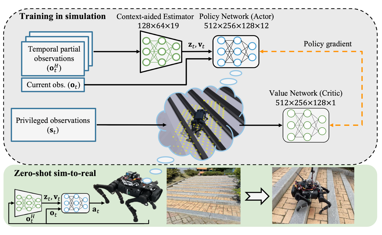
DreamWaQ, KAIST
41:38–> 42:38
So instead what they do is they have a second output head from their policy. Their primary output head is controlling the robot, but the second output head is predicting what the height scan around the robot looks like, and in simulation, of course, you can access this.
And so it means that on the real robot, even though this is a fully blind policy, usually for these small quadrupeds, they struggle with stairs when blind, because they’ve got to pick their feet very high up. Through interacting with the environment, it’s able to estimate that there is a stair here, and navigate that even without explicit observation of the environment. That’s pretty impressive.
People also do this for, uh, linear velocity as well. So, as opposed to learning an explicit estimator of linear velocity, this is one way to get it implicitly, by training the network to have an additional output head to estimate linear velocity.
And if that converges during training, then you can argue that the weights of the latent space of the neural network has sufficient information to reconstruct the linear velocity.
42:38–> 42:48
Which you never actually need explicitly, as long as you’re confident that the policy knows about it and can reason about it and act accordingly. This can help with efficiency, uh, to help boost trap learning in sensor-denied environments as well.
53:38–> 54:38
So, next we’ll talk about curricula. Uh, they’re not strictly necessary, and there’s not a good science for how to do them yet, other than a few canonical examples that we’ll discuss.
But they can be really, really helpful when you have a hard task, that you’re finding the policy struggles to learn. This is especially true in manipulation. I think curricula are a lot better understood for manipulation than they are in locomotion.
For locomotion, the most common example of a curricula is your terrains. So you can see in this image, sort of at the left side of the image, we have these very steep pyramids and steep pits and high variability in the step height.
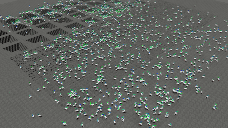
But if you look all the way to the left, then it’s much, much flatter. And so part of what we do with these curricula is we start with an easier version of the task, such that we can define a programmatic way of increasing the difficulty of the task as the policy learns. So as the policy becomes more capable, we should make the task harder until we get to the task we actually care about.
When we want to do, let’s say, stair climbing, you don’t start with stairs, you start with flat ground walking.
54:38–> 55:38
And then introduce stairs as you go throughout training, higher and higher stairs, until you’re doing the tasks that you care about.
And as a simple heuristic, if you define some success metric, in this kind of terrain-based environment, it’s usually the total distance traveled from reset. But if you find you get more than 75% success, then you should increase the complexity of the task and put the robot in a more difficult environment.
If you’re getting less than 50%, then maybe bump it back down to the easier environment so it can practice there. And so you can see that for this somewhat flat ground, where you just have the steps or the random variation. In this example, they have robots spanning the entire terrain space. In these much harder pyramids and pits they’re very much overrepresented in these easier levels, but the policy has not increased in capability enough yet to put it in the harder parts of the terrain.
So you update that programmatically, and various simulators have ways of dealing with this. Isaac in particular, has a nice curriculum interface for this.
55:38–> 56:38
Then another example of this was the Spot running demo. This was the other intern that I worked with, AJ Miller. And his work was in getting Spot to run at over 5 meters per second. The stock controller from the factory could do 1.25 meters per second, the fastest that I think they had ever seen internally at BD was 2.25 meters per second.
So we were able to over-double that. And a big part of that was the velocity curriculum. If you tell the robot when it doesn’t know how to move at all, that you want it to go 5 meters per second, then you give it a really big penalty, or basically no reward signal at all. And it’s very hard for it to learn that way.
And so instead, we started by asking for it to walk at up to 1 meter per second, and as it got better at that speed, then we asked it to go up to 2 meters per second, and then 3, and then 4, etc. So as the robot became more capable and gained skills, we asked it to do harder and harder tasks, to converge on the task we wanted, which was to maximize its velocity. But you don’t start with that version of the task immediately.
59:28–> 1:00:38
Now just a little bit on reward tuning and tuition.
This is also very much an art and not a science, so I’ll give you my perspective on it, what’s worked well for me. Other people may have totally different perspective on it, but I tend to approach reward tuning as a control theorist, more than as a strict learning person.
I think learning people tend to, uh, prefer sparse rewards, you know, success metrics, things like that. I think it’s oftentimes more helpful in legged locomotion to treat this as the cost for MPC. They’re not the same, obviously, their intuition is distinct. But I think it’s easier to start from that place of intuition and build on it into the learning side, then vice versa.
And so I want one more question real quick before I jump into that.
01:00:38-01:01:38
The general way that I think about it is that the weight loosely encodes the order that you want to be learning your different tasks. So if you have some very large, high, positive weight rewards, those are the things the policy will learn first. Because it’s going to drive TD error, so the critic will try to resolve that and guide the policy to minimize TV error, and that’s what ends up being learned first as a skill.
When it’s possible, and it’s not always, but when it’s possible, try to factor rewards into somewhat independent actions. So, for example, while my foot clearance, while the height of my foot is above the ground, it’s certainly dependent on how fast I’m going in some sense.
01:01:38 –> 01:02:38
I can tune them as independent knobs. I can say, oh, I’d like to walk at 1 meter per second, and whether I’m picking my foot up 10 centimeters versus 15 centimeters from the ground, that’s sort of independent of my choice of desired base velocity.
They are coupled through the dynamics, but you can think of them as being independent in the sense, as opposed to two rewards that maybe are more intimately tied.
In general, I split all of my rewards into task rewards versus penalties. So your task rewards tend to be large and positive rewards that define the bulk behavior. If you squint, what is the robot doing? Is it velocity tracking? Is it navigation? Is it goal? Is it reorientation about some goal? Etc.
It’s pretty common to do, like, a squared exponential or a normed exponential as the kernel for these. So it looks like a bell curve, so it gives you a nice, smooth gradient to minimize some error. Usually you define an error for your task, and then you have this squared exponential to minimize it with a positive reward.
01:02:38 –> 01:03:38
People occasionally will also use the L1 kernel instead of L2 for the exponential. That gives you more of the absolute value if you were to plot, you know, the E to the negative absolute value of X. You get a much spikier function.
You don’t want all of your rewards to look like that, because you’ll end up with a lot of jitter, because the policy can never converge on a low error state. Because it’s so spiky. But for some rewards where you really want to make sure you push it to minimize err as much as possible, it’s a much more aggressive kernel.
So an example of that might be if you’re trying to minimize error between some desired base height for your robot, you typically want to use an L1 kernel instead of L2, because you’ll get much more high-fidelity tracking, but it isn’t the dominant task reward, your velocity tracking usually is.
And so you’re able to avoid the kind of jitter you might see if you only use L1 exponentials. While still getting high fidelity tracking performance. And this is some of the reasoning there.
If you look at that compared to the inverse, the inverse is 1 over 1 plus X squared, where you’re trying to minimize X squared, that is almost the exact same shape as a bell curve.
01:03:38 –> 01:04:38
So a lot of these have very, very similar shapes and characteristics. And currently, squared exponentials are the kernel that people most typically use.
For regularizing penalties, this is just minimizing some L2 norm, so minimize energy usage, minimize joint accelerations, minimize violations beyond your desired joint limits if you’re not enforcing them as a strict penalty, or as a strict termination condition.
These typically have much smaller weights. And the idea is that you start by learning all of your task words, you enforce that the policy will learn the bulk behavior that you want, but it might look a little ugly doing it. At that point, your mean total reward typically converges, because most of the reward that you’re getting is coming from these large positive task rewards.
And then you let it train for 2 to 5 times longer than it looks like you need to, longer than it looks like it’s converged. And that’s what really gets all these regularizing penalties to shake out the behavior to make it much, much smoother.
I very often see, when you look at more learning-style papers of the Atari games, whatever, they’re trying to maximize their success rate.
01:04:38 –> 01:05:38
And the minute that they get the high enough success rate that they want, they stop training. For us, when we’re trying to deploy this on real hardware, you typically want to train it a good deal longer than that, because the result is a much, much smoother policy, and this goes back to where the policy’s learning from.
It’s not just that you’re trying to maximize your rewards, but it’s specifically that you’re trying to minimize the temporal differencing error from the critic. Without going too much into the theory, all that means is if the critic can expect the reward or penalty, then it’s not going to learn from it.
And so, early in training, all of the error between what the critic expects and what’s actually happening is coming from these high-magnitude task rewards, but later in training, when it looks like the reward is converged what’s actually happening is there’s still TD error coming from the critic for these smaller magnitude regularizers.
And minimizing that takes a lot longer than you’d expect. And so, usually, for the rewards I have tuned, when I deploy them on hardware, and this is true whether Quadruped humanoids or across modality, I’ll train for 20,000 to 30,000 iterations.
01:05:38 –> 01:06:38
You can minimize that if you have a lot more parallel environments. When I do that, I usually have about 4,000 environments, which works well on consumer GPUs. But if you have a nice server rack of H100s burning a hole in your pocket, then, yeah, go to 32,000 environments. Train on multi-GPU, and you’ll converge much, much faster. And by faster, I mean in fewer number of iterations.
But you still do want to let it converge and then sit there for a while to get the nice SIM-to-real transfer.
Then last note here: ensure that you always have a net positive reward, uh, otherwise, if the net reward is negative and the robot has some way of terminating the episode, for example, by making contact with the ground, it will learn to kill itself. If life is suffering, then there’s an easy way out.
Instead, if the reward is always net positive, then it will never do that. It will always learn the task that you want, or at least it will learn to maximize the length of the episode, because there’s always positive reward to be had. I often see people using a termination penalty to try and prevent this from happening.
01:06:38 –> 01:06:38
I find it much harder to intuit and tune when termination penalties are applied, and so I typically prefer to use a live rewarder and a live bonus to push the net reward to always be positive at the beginning of training, to make sure that the robots don’t learn early termination.
01:17:08 –> 01:17:38
Okay, so next, some commons. So, you asked about the common rewards. This is very similar to what we see in the paper that was linked in the chat from Spot running, and you can see it’s very clearly split into task rewards, which are positive, versus the penalties, which are the negatives.
I’m not gonna go into these explicitly, just in the interest of time. They’re fairly straightforward and somewhat uniform in the literature.
I will say that, again, as reward tuning is more of an art than a science, there are small changes, for example, the L1 vs. L2 kernel, that do make a big difference.
01:17:38 –> 01:18:38
It doesn’t seem like it should, but that choice can pretty drastically change how smooth your resulting policy is, and that’s mostly a matter of trial and error. So I, at this point, like I mentioned, I’ve got this set of rewards that I really like that works well for me, so I use them everywhere.
But to get those rewards, there wasn’t really any first principles reasoning to get there. It is fairly empirical and heuristic. It takes practice on your robot to get the right formalism and weights and kernel for your robot specifically.
But these are the general things, the parameters, the knobs I like to have to be able to tune, to be able to get the kinds of behavior that I want for legged locomotion.
And of course, this is a velocity tracking formalism, but you can swap this to navigation pretty easily just by changing out some of the task rewards.
Okay, I would say, the most important, uh, parameter in all of training for RL. When we train our policy,the policy doesn’t actually give us an action, it gives us a mean and a standard deviation.
01:18:38 –> 01:19:38
So we can parameterize some multivariate Gaussian that we sample, and that’s where our action comes from.
At runtime, we’re just taking the mean of the distribution, but for training, the standard deviation is vitally important to be able to do this sampling procedure. When you are training, first and foremost, make sure that you are logging the standard deviation. If you are not logging your standard deviation, you do not know how well your robot is working, doesn’t matter what the rewards look like, doesn’t matter if your loss converges.
If you don’t know your standard deviation, you don’t know how good your policy is. Once you do have your standard deviation logged, make sure it is decreasing. It should not go to zero, but it should converge from whatever its initial value, usually 1, to some smaller value. This is the most important thing to do your RL tuning.
If this value does not converge, nothing you do matters, because the policy does not know the effect of its actions. The standard deviation is the policy telling you how confident it is that its action is going to be a good one.
01:23:38 –> 01:24:38
And then last, just to finish up here, let’s talk about RL with Motion references, because they’re becoming very popular. I think for good reason. If we want to think about task specification as a spectrum, on one end, we have behavior cloning, we have an exact teleoperated example of what we want our robot to do, and we’d like the policy to exactly mimic or clone that behavior. We have fully specified our task, it is very, very rigid, but we have a great deal of control over what the robot does, because we’re just showing it.
On the opposite end of the spectrum, you’ve got the vanilla RL formalism, especially when you only have a few rewards where you aren’t over-prescribing your rewards. You have a very, very flexible task specification. If your only reward is track velocity and minimize energy, then the robot will find whatever unnatural gate to be able to do that. But it’s got maximum ability to explore and flexibility to achieve the task.
01:24:38 –> 01:25:38
In practice, though, we don’t want the most flexible version of this, because we know from first principles how our robot should behave. We’ve got some desire for what that motion looks like, how smooth it is, etc.
And so you can increase the specification of the task. Either by adding more rewards by hand or, what’s even easier to do is to use motion references. And so these motion references, as we see in this video, give the robot a sort of more in the style of behavior cloning, a reference for what it should do, its joint angles, its base, you know, state, etc.
But because you’re still training it with the reinforcement learning formalism, it has a great degree of robustness to things like ground friction, or center of mass, or if different inertial properties, things like that. Then in behavior cloning, if you go out of distribution, where you don’t have data, you expect performance to degrade rapidly, whereas with RL, because we can generate data at train time with this wide variety of real-world conditions.
We can start with fairly simple and very small amounts of reference data, and expand that into a very robust policy that works on hardware.
01:25:38 –> 01:26:38
So it’s part of why we’re seeing it work so effectively. There’re two main different ways to do this, either GAN or discriminator-based versus feature-based. So, AMP, Adversarial Motion Priors, is the canonical example of GAN-based. It’s very scalable to diverse environments, you’re just estimating the style, or you’re trying to mimic the style of the distribution of your reference data.
But because it’s a discriminator trained in parallel with the actor, it can be very difficult to train and hard to interpret. Just in general, I feel like the intuition for training discriminators is quite difficult, even though they work well in practice once they’ve been trained.
Compared to feature-based, this is more like training an auto-encoder on your reference data, and then using latent conditioning to get the behavior you want.
This tends to be much easier to train and interpret. You can get nice compositionality with it. The motion imitation itself is much higher quality and higher fidelity, much lower joint tracking errors, for example. But it doesn’t generalize nearly as well.
01:26:38 –> 01:27:38
So depending on your task, whether you’re trying to mimic one specific behavior that you want to have high fidelity on, you would use feature-based. Versus if you just want the style of natural gait walking, for example, then GAN-based is gonna typically do better for you in that setting.
And then, just to wrap up, summary. Lower PD gains will give you better exploration and you should enforce everything as a soft constraint. The hard constraints will hurt you. If you start with a perfect model, then you know the capabilities of your task setup and your rewards, and then you add realism iteratively until you converge on your real system model.
You should train a lot longer than you think and use less domain randomization than you think.
Please, use a state estimator, your life will get easier, I promise.
The hyperparameters that you get with PPO, generally, at this point, are good. We call them Nikita magic numbers, because they are tuned well, and they work.
But the most important takeaway, I hope, that you got from this talk: there is no replacement for principled system identification.
01:27:38 –> 01:28:38
If you have a good and well-identified system, RL is not hard. If you are struggling with RL, most of the time when I’ve seen this at various labs, it is because they do not have good system identification. This is the most critical thing to make RL work in practice, the difference between “drunken robot syndrome” versus the really, really smooth and slick demos is system identification. The better you know your robot, the better RL will treat you. And so I think teams that spend the time and effort to do good system identification will be rewarded with better performing RL, and that’s the most important thing I could possibly impart.