Gyre: Scaling Manipulation With Real-World RL


Rationale
Industrial automation sets an unforgiving bar. To take over a station on a real production line, a robot has to repeat a task thousands of times a day, at human speed or faster, and almost never fail. The target we hold ourselves to is 99.9% success at human or superhuman speed, reached predictably enough to plan a deployment around it.
We have bet from the start on end-to-end deep learning to clear that bar. Vision-Language-Action models (VLAs) are the strongest architecture for it today, and they sit at the core of our stack. The dominant way to train them is behavior cloning (BC): collect demonstrations, then train a policy to reproduce them. BC has produced strong results, but on its own it runs into ceilings that keep it short of industrial deployment.
First, speed and quality are capped by the demonstrator. A policy trained on teleoperated demonstrations inherits the speed and the quality of the data it was trained on. The naive fix for speed is to replay the learned behavior faster, but physics gets in the way. Actuators have finite dynamics: a gripper closes at some maximum speed, a joint accelerates at some maximum rate. Run the policy faster and its timing assumptions stop matching reality, so the arm begins to retract before the grasp has closed. In our previous post we introduced a data-side “sport mode” that speeds the policy up at training time to address some of these issues. It is a heuristic, though, with inherent limits, and it fails if pushed too far. To go faster and cleaner than the demonstrator, the policy has to learn directly from physical interactions.
Second, passive imitation does not reach industrial reliability. Industrial deployment demands near-perfect reliability, with interventions rare enough that the fleet essentially runs itself. BC struggles here because it only imitates good behavior and never sees the cost of bad behavior. The policy learns what to do and learns almost nothing about what not to do. That gap matters most where it is most dangerous: when a bad action turns into a safety problem.
BC is also prone to causal confusion [1]. A VLA policy acts on far less information than the operator who produced its data: the operator carries long-term memory the policy may lack, brings far more computation into a decision than a single VLA forward pass allows, and potentially sees the scene through a different viewpoint. When these drivers of the demonstrated action are invisible to the policy, the true cause of success can be hidden, and imitation may latch onto whatever visible signal correlates with it instead. The policy can look perfect in familiar scenes, but fail the moment that correlation breaks.
Reinforcement Learning (RL) addresses both ceilings directly. RL learns by trial and error against an explicit reward, rather than by copying. It optimizes for task performance inside the robot’s real physical dynamics, the same actuator limits and contact physics the deployed policy will face. Because RL is not bound to the demonstrations, it can push past the demonstrator in both speed and quality. It also corrects causal confusion and other failure modes directly: a policy leaning on a spurious correlate eventually fails the task, and RL detects and suppresses that behavior, driving down the long tail of failures rather than hoping they were absent from the training set.
RL is the path to general industrial robotics, and we are building our stack around it. We already rely on it at the System 0 level for whole-body control. Gyre extends end-to-end, vision-guided RL up the stack to System 1, the manipulation VLAs.
Running robot training 24/7
Getting RL to work on top of a modern VLA stack is hard, both technically and operationally, and there is no ready-made playbook for it. We had to write our own; we call it Gyre. This section describes the challenges we hit, and the solutions we adopted: setting up the training infrastructure, adapting PPO to flow-matching VLAs, keeping the robot safe under exploration, and holding training stable as speed ramps up and the real environment drifts.
Sim-to-real or not?
The first decision in setting up RL is a fundamental one: where to run it, in simulation or on the robot. We do both, for different purposes.
Simulation has one clear advantage: it scales with compute, so we can spend much more robot-hours in sim than on any fleet of physical robots. Its limitation is transfer: moving a policy from sim to the hardware zero-shot means closing the sim-to-real gap, and doing that faithfully (the end effectors, the objects, the way they make contact) is still challenging to scale across many environments with different assets. The choice also has to fit our deployment plans: we want fleets to keep learning after they ship, turning supervisor interventions into rewards. This is why we run RL directly on real hardware: there is no gap to close, the policy is optimized for the dynamics it will be deployed under, and the training loop we run today is the same one we will run at customer sites.
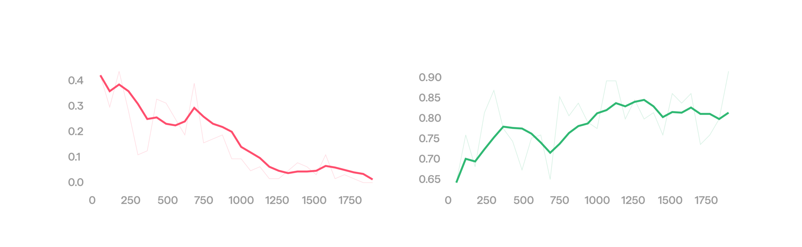
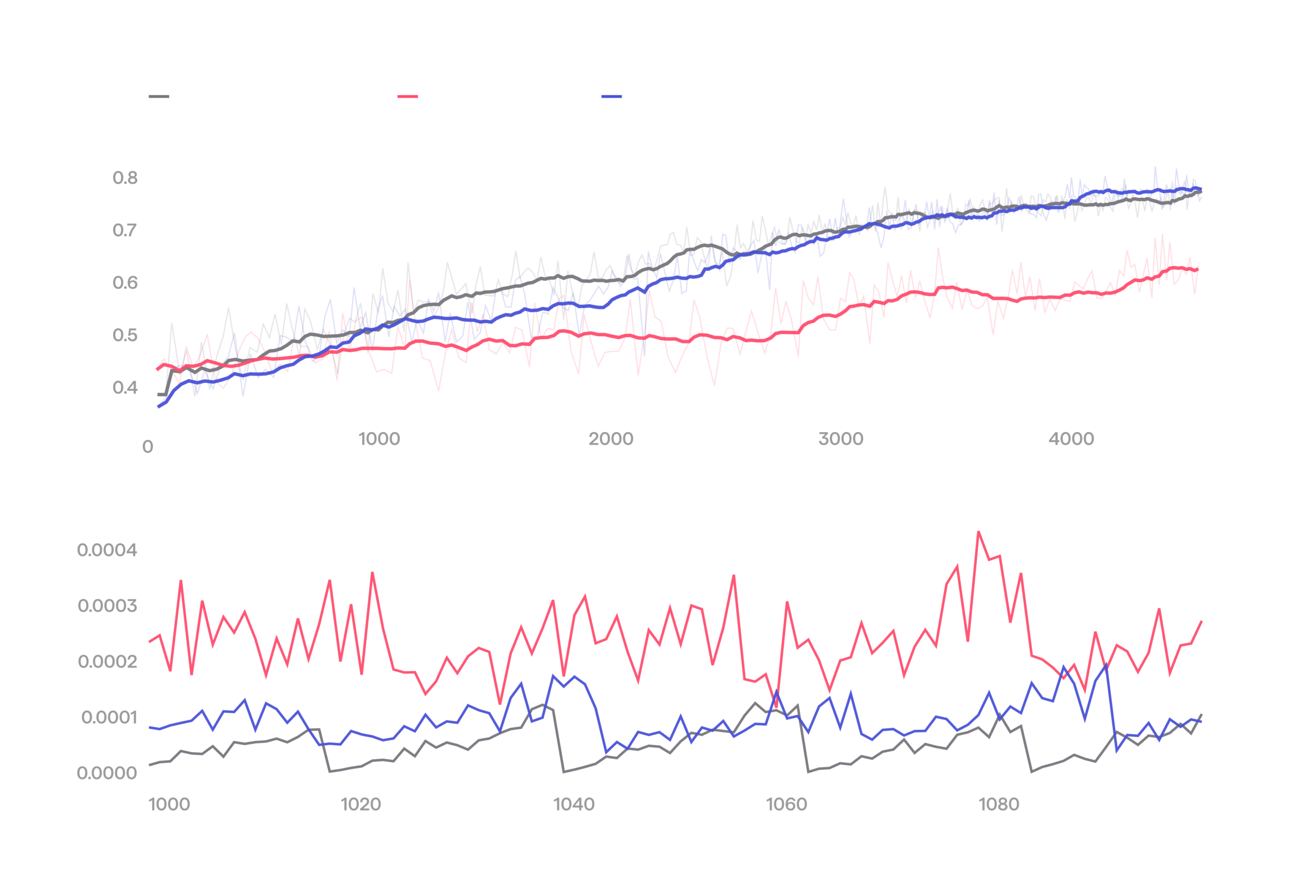
That said, we use simulation heavily. Our work on RL methods and sample efficiency is done in sim, where iteration is fast and cheap. We keep digital twins of the physical environments, and in simulation we now routinely reach 100% success rates on those. RL performance in sim and on real hardware also turns out to be closely correlated. The plot below shows reward (which in this case is basically success rate) over the course of training for the same task both in simulation and on the real hardware.
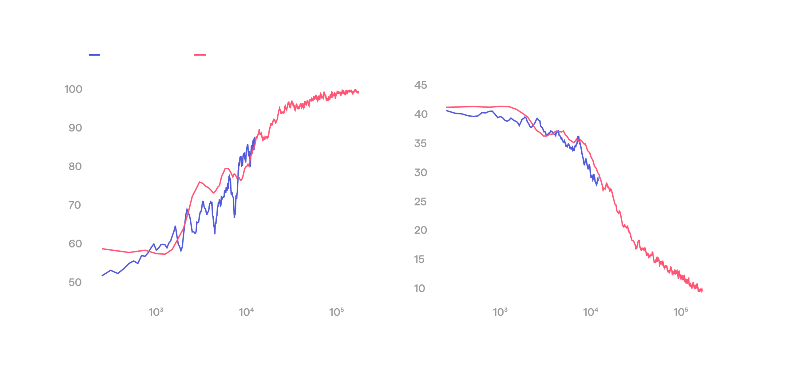
RL follows the same scaling trend in sim and on real hardware.
This plot shows two things. First, training dynamics in sim and real match closely: the real curve tracks the sim curve over the range we have run so far. Second, and more importantly, the real run sits on the same trajectory that carries sim to 100%. We read this as direct evidence that full reliability on real hardware is a matter of robot time and compute, not of missing methods. This figure is the basis for the claim we opened with: we now have line of sight to our reliability target.
Disaggregated training and rollout infrastructure
A single facility can have hundreds of robots operating at once, and streaming that many real-time camera feeds out of the facility to a nearby GPU datacenter is not feasible. This is why we run inference onboard each robot, currently relying on NVIDIA Jetson Thor as a compute platform. The RL stack has to work within the same constraint. It needs to collect rollouts on the edge devices and stream updated weights back to the edge during training. It’s also important to roll out episodes on the hardware the policy will eventually be deployed because the same policy might produce slightly different actions on different devices due to numerics (we revisit this point in the [Sampler-trainer gap correction] section).
For these reasons, our RL training infrastructure fully disaggregates training and inference hardware. The trainer holds the policy and runs the updates on the server, and rollout collection is delegated to separate workers behind a thin interface. A worker connects to the server, pulls the current weights, runs rollouts, and sends the transitions back. A worker can be a Jetson on a robot or a simulator instance in the cloud; the server communicates with both through the same interface. Throughput scales with the number of attached workers. A single training run can collect rollouts from physical robots and simulation at the same time, a sample efficiency improvement direction we are keen on exploring further.
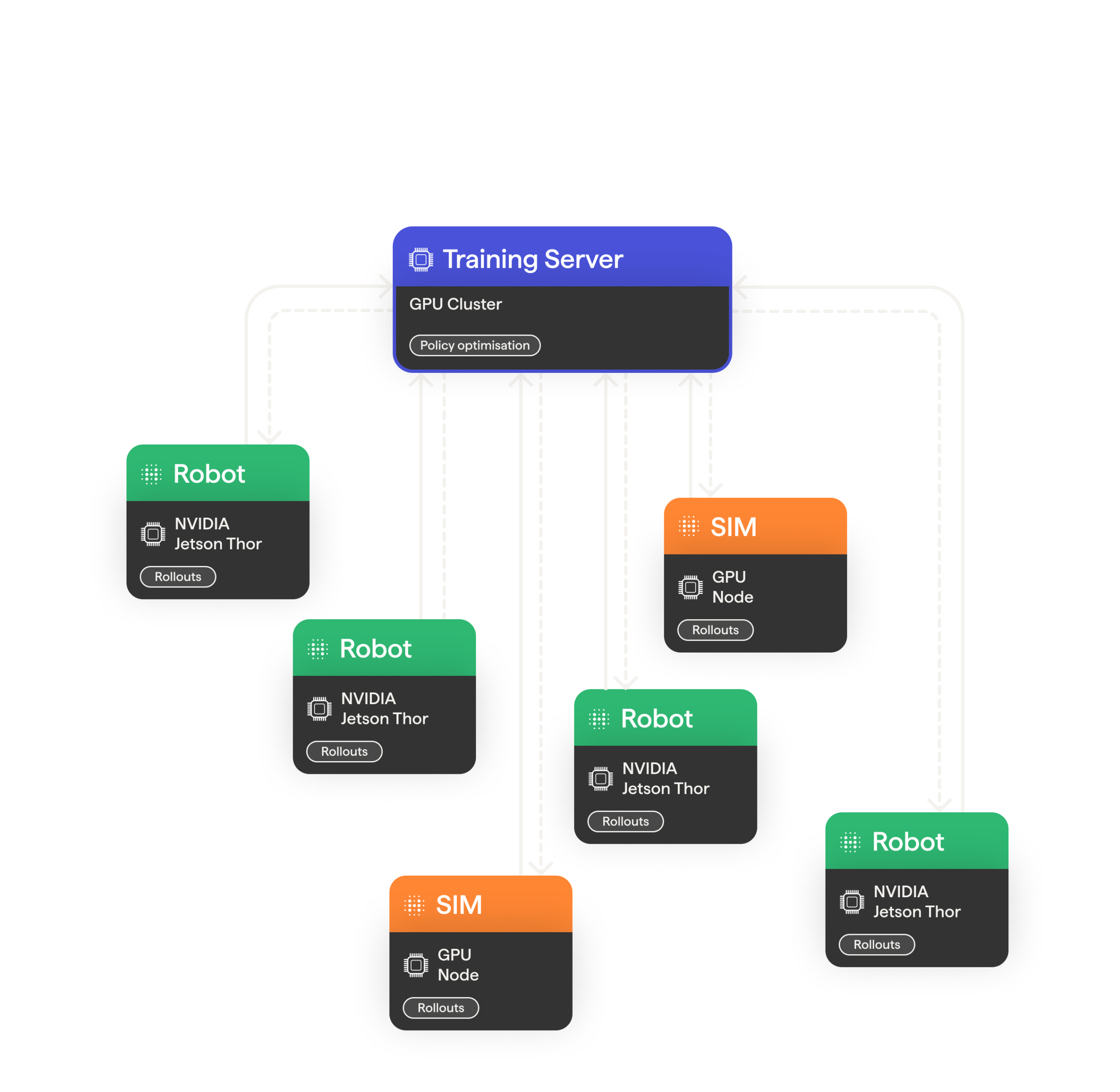
Distributed RL training infrastructure: Thor-powered robots and simulation nodes produce rollouts and receive policy updates from the training cluster.
PPO with CFM-based policies
Our manipulation policies are based on conditional flow matching (CFM) [6] and trained with behavior cloning. Flow matching has proven to be an efficient way to model the complex, multimodal distributions over action trajectories that manipulation requires, and it sits at the core of some of the strongest VLAs to date, such as Physical Intelligence’s π0.5 [7] or NVIDIA’s GR00T N1 [8]. Since our own VLA stack is also built on CFMs, getting RL to work reliably on top of CFM-based policies was a priority for us: switching to a policy class that is easier to train with RL would mean giving up on CFM benefits.
A CFM policy samples an action by drawing a noise vector and integrating a learned velocity field, a deterministic ODE [6]. Doing RL on top of it requires to know the probability the policy assigns to each sampled action, and computing this probability exactly is impractical during RL training. The standard fix [5] is to convert the sampling ODE into an SDE by injecting Gaussian noise at every integration step. Each noised step then has a tractable Gaussian density, which gives the per-action log-probabilities we need, and the noise doubles as an exploration driver.
Several published methods applied RL to flow matching this way. We tested some of them extensively in sim, but each method fell short at our scale and task difficulty. Full ablations are out of scope here, but briefly:
- ReinFlow [10]. Zero to modest improvement at our scale, unstable.
- Flow Policy Optimization [2]. Worked on our simplest manipulation environments but not on the harder ones.
- Flow-GRPO [5]. Worked on our industrial tasks but was extremely sample-inefficient.
- Reinforce Adjoint Matching [3]. Behaved like Flow-GRPO, without the sample-efficiency gains it advertises.
Eventually we have converged to a PPO-based approach closely resembling Flow-SDE [13], which strikes a good balance between sample efficiency, training stability and hyperparameter robustness.
Similar to [13], we found that PPO paired with the ODE-to-SDE conversion works best, giving consistent improvements across all our simulation environments under a single hyperparameter set. We also confirmed that injecting noise at one randomly chosen integration step performs well while keeping training fast. Additionally, we always leave the last integration step noise-free to reduce action jitter. We follow the same noise schedule as [13] and [5], setting noise to the highest level that does not noticeably degrade the policy.
We run PPO with a regression-based critic, for accurate credit assignment. Value estimation is much more tractable in motor control than in, say, reasoning: in our experiments, learning an accurate critic for a manipulation task was not hard, which is unsurprising given that evolutionarily ancient, simple circuitry in biological brains can do it well. Lack of accurate credit assignment is likely part of why the critic-free methods above, such as Flow-GRPO, were so sample-inefficient for us. During training, we maintain fully separated policy and critic weights, both initialized from the same BC checkpoint. The critic reads a trainable CLS token through a linear projection to produce its value estimate. The objective is the standard clipped PPO loss with GAE, plus the prefix-CFM term described in the next section.
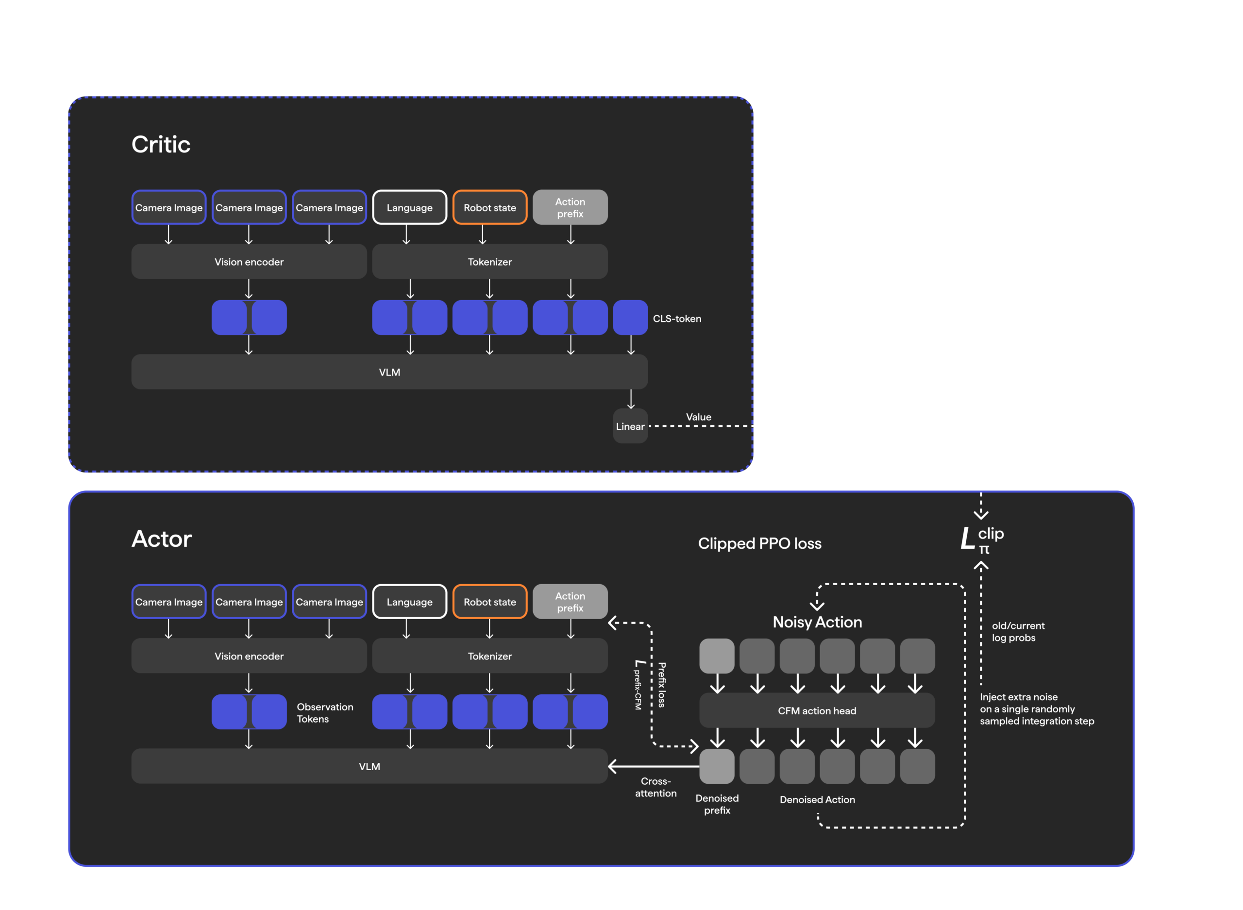
Model architecture and RL training objective.
CFM prefix loss
We normally train our models to predict two second long action chunks with actions sampled at 30 Hz. During normal operation we execute only the first 200 ms of each chunk before replanning, but predicting further ahead leaves enough slack to absorb latency jitter, or to run the same policy on higher-latency inference hardware. Learning to predict further into the future also generally helps model performance.
To avoid jerks at chunk boundaries, we use asynchronous inference with action prefix conditioning, introduced in our previous post. We feed an extra input into the model: the slice of the current chunk that will be executed while the next chunk is being prepared. This slice is what we call the prefix. During BC the model learns both to copy this prefix into its output and to continue it smoothly into the future. Unlike the closest published approach [9], prefix conditioning works for any action head architecture, because it relies purely on conditioning and not on features of flow matching.
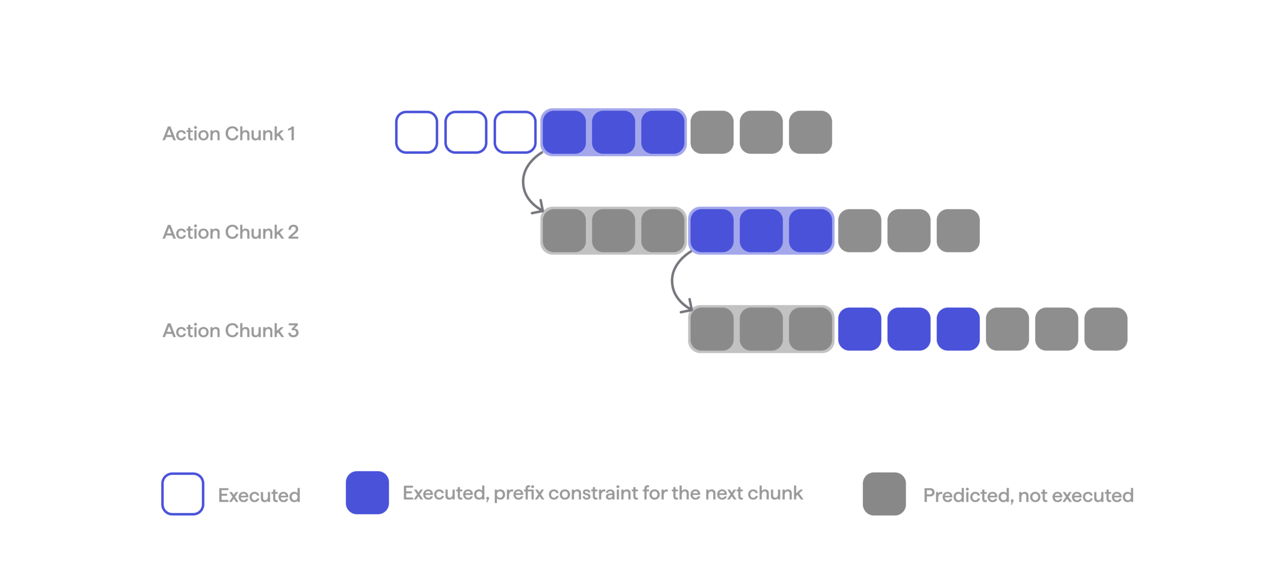
Prefix conditioning during BC training.
Under RL training, prefix copying quietly breaks down. RL rewards only the actions that actually execute, never the copied prefix, so nothing holds the model to reproducing it. Free of that constraint, the policy starts violating chunk transition smoothness to raise reward in the short run. Over a longer run this behavior sets off a feedback loop: the prefix for the next chunk is taken from the previous chunk’s prediction, and so as the prediction drifts, the prefix fed back in as conditioning goes out of distribution; the OOD input in turn pushes the next prediction further off; and the drift compounds from chunk to chunk. One way this effect manifests is a slow drift in the joints not doing the task, like the idle arm or the torso. Once the inputs are far enough out of distribution, oscillations appear, and eventually training diverges. We have not seen this failure mode described elsewhere, but expect any RL setup with similar action-prefix conditioning to eventually hit it.
Arm drift after long RL training caused by action prefix drift
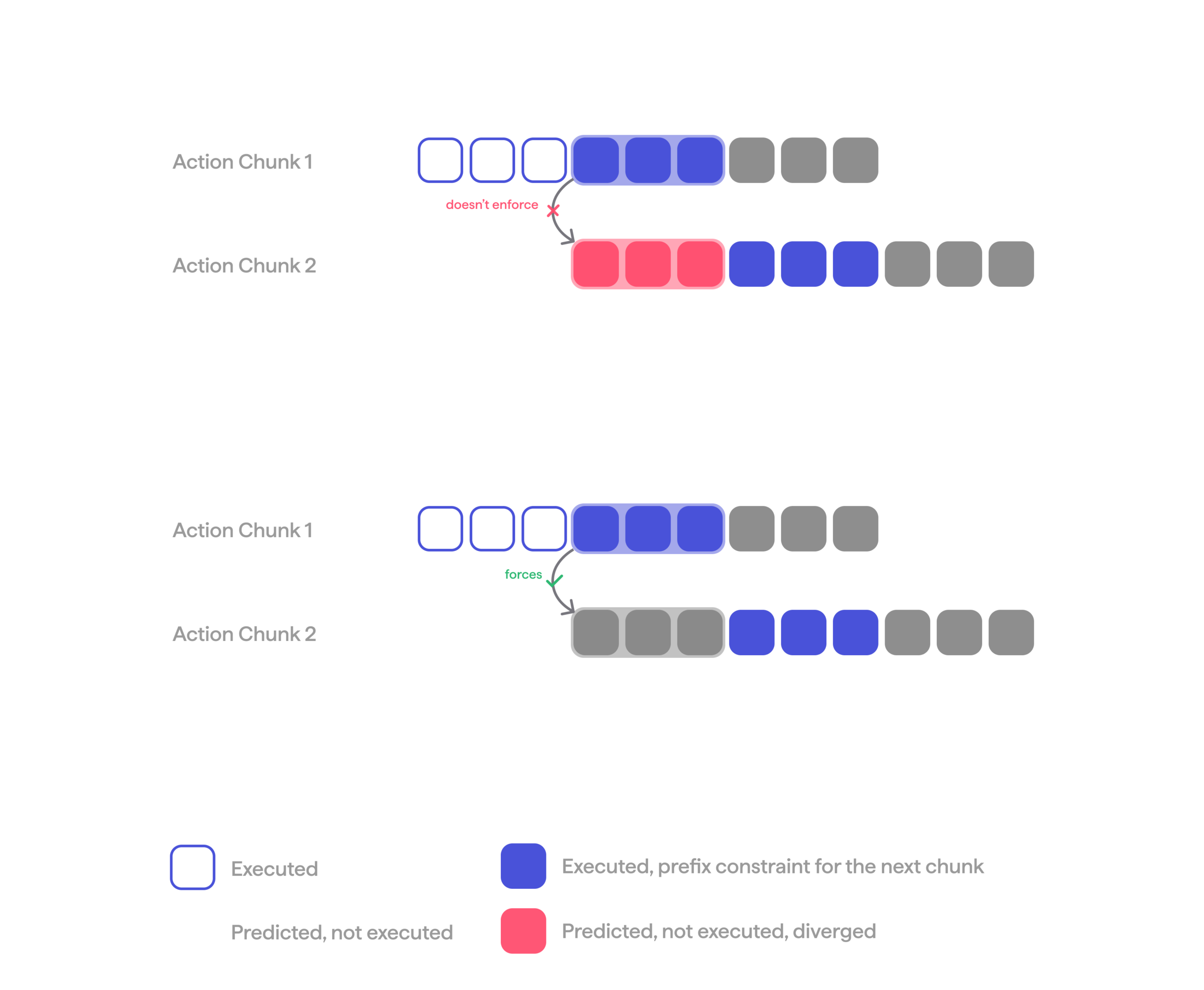
RL training with unconstrained vs constrained prefix.
This issue can be fixed by adding an extra loss term to the PPO objective that encourages the predicted action chunk to start from the provided prefix during RL training. We apply this term to all chunks regardless of associated rewards since this property should hold universally. Our final training loss therefore takes the following form:
– clipped PPO policy loss
——–
– value loss
– masked CFM regression loss on action-prefix slots
—
– value loss weight
———-
– prefix CFM loss weight
The plot below demonstrates the evolution of CFM prefix loss and inactive arm drift over the course of an RL run. In the vanilla run with prefix loss disabled, the prefix loss tracks the drift and peaks exactly where the drift is worst, near the end. Enabling prefix loss prevents the drift, keeping the run stable.
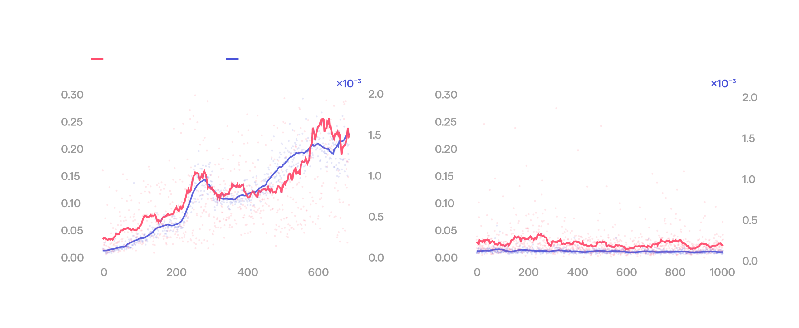
Idle arm drift and prefix loss before and after introducing CFM prefix loss.
Keeping hardware safe under exploration
Our applications are hard on the hardware. We operate with heavy objects and run 24/7, which compounds the wear. Collisions and large forces are routine. Exploration makes it worse: during RL the robot must try new actions, some of which are damaging. So a major part of our RL effort goes into preventing breakage.
Active compliance is our first line of defense: on unexpected contact the arm yields and reduces the contact force. But it can only do this within the joints’ range of motion. Once a joint reaches its travel limit, the force is transmitted directly into the structure — and this is where the robot can experience mechanical overloading. That is precisely where an additional safeguard is needed. One way to stay within range is to raise the controller stiffness for a given task. But stiffness trades directly against compliance — the stiffer we make the arm, the less it absorbs in the first place — and tuning it per task only addresses the cases we anticipate, not a general solution.
For this reason we added a second, independent safeguard on top of controller compliance. We monitor the wrench applied at the wrist and halt execution the moment the measured force crosses a safe threshold. We then replay the recent commands in reverse to retract the arm quickly, a pain-like reflex.
Safety termination during ring picking
Auto-termination based on force-torque signal
Finally, since episodes terminate on safety violations, we implicitly train the robot to minimize the number of safety-triggered stops. Behavior cloning alone cannot achieve this: we do not want to copy demonstrations that use excessive force, and an imitation policy can only react to force that is already applied. RL learns to prevent applying excessive force in the first place, and over a run we see the reflex trigger less and less often.
The rate of safety terminations declines during training, allowing success rate to grow.
Reward design
Reward design is an important part of RL setup. It is also one of the scaling bottlenecks of universally applicable RL training.
One approach is to shape the reward with many terms that give the policy dense, step-by-step guidance. Dense shaping helps with credit assignment, but requires task-specific experimentation that doesn’t scale well to many tasks. The resulting reward can also be fragile: with many interacting terms, the policy often finds non-obvious ways to exploit shaping. Finally, reward shaping might require access to privileged information (e.g. object location) that is not easily available when training in the real world.
We keep our rewards sparse and generic. The core signal is a single binary reward for task success, such as a completed pick. We do not add a dense term to encourage speed: reward discounting already supplies the time pressure. We still add sparse penalties for common types of failures we can detect easily, such as a misgrasp, because penalizing them explicitly helps credit assignment. Safety enters the reward implicitly: an episode terminates on a force threshold violation, so unsafe behavior is automatically disincentivised (see [Keeping hardware safe under exploration]).
None of these terms are task-specific, so setting up training for a new capability is straightforward: we define success, what recoverable error types we want to penalize explicitly, and rely on discounting to create optimality pressure. That keeps the approach practical to apply across many tasks.
——-
– reward for task success
– recoverable error penalty
———–
– recoverable error penalty weight
Non-stationary real environments
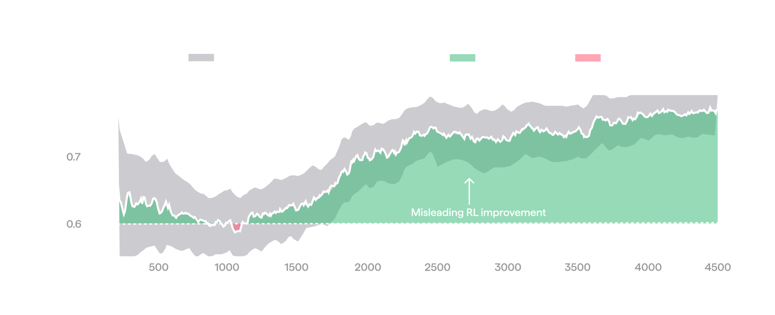
It is tempting to treat the reward at the start of an RL training run as a fixed baseline and credit any rise above it to training progress. For example, the run below looks like a clear win: reward starts around 0.6 and ends up much higher, around 0.75.
Misleading RL improvement against a stationary baseline.
In real environments, this assumption is violated: they can drift over time, so a fixed point is not generally a good reference. To track the baseline as the environment drifts, we unroll a small fraction of episodes (around 10%) with the frozen reference policy (e.g. the pre-RL starting policy) instead of the current one, using reference episodes only for monitoring. This is a form of online A/B testing. Plotting rewards within the same window together with the A/B baseline paints an entirely different picture for the run above: the baseline rises just as much as the RL policy, so RL produces no real improvement in this run.
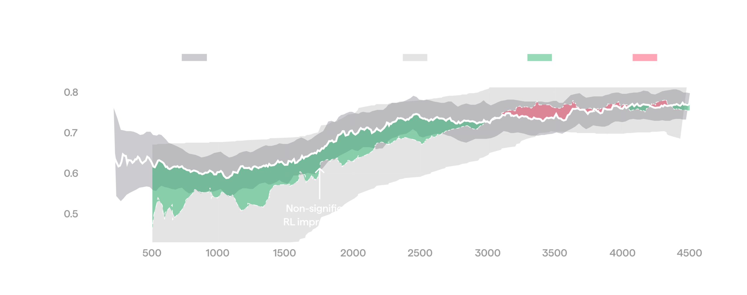
When comparing against a moving baseline, improvement vanishes.
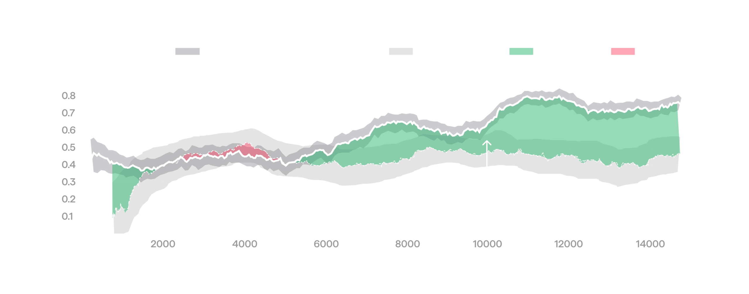
The plot below shows a successful run where RL pulls clearly above the baseline, and the advantage widens as training continues. Every gain we report in this blog post is measured this way: against the concurrent baseline in A/B fashion, rather than against a stale one.
Real improvement against a moving baseline.
Here are some common factors that can drive environment non-stationarity:
- Image brightness, which changes over the day/night cycle. We often run around the clock, so the lighting is constantly shifting.
- Operator shifts. Different operators can have a slightly different understanding of operational instructions, leading, for example, to operator-dependent biases when resetting the environment.
- Wear and tear. Hardware might accumulate damage during operation, gradually reducing performance.
Sampler-trainer gap correction
In PPO, each gradient term is weighted by the ratio between the probability the current policy assigns to an action and the probability the action was sampled with. An error in this ratio translates directly into an error in the update, which might easily lead to divergence. In our disaggregated RL stack, training and inference are performed on different devices: actions are sampled on edge compute and the gradient is computed in the cloud. Running the same weights through these two paths yields slightly different results, and the probability a rollout worker reports for an action differs from the one the trainer computes for it. We call this discrepancy the sampler-trainer gap.
Sampler-trainer gap has several causes, some of which are hard to remove. The largest is hardware: our rollouts run on NVIDIA Thors, while training runs on Hoppers and Blackwells, platforms with different compilers, kernels, and dedicated code paths. The two stacks can differ in numerical precision of some operations and call kernels, whose output depends on batch size. We also optimize our inference stack for latency aggressively, which widens the gap further.
Sampler-trainer gap can be closed by making training and inference numerically consistent by using batch-invariant kernels, aligning dtypes and compiler settings, and reusing the same kernel implementations wherever possible [11]. We can do this only partially, because our action sampler is pinned to the production inference stack, so that RL always trains under deployment conditions.
We therefore correct the gap on the trainer side. Instead of using action probabilities reported by the inference stack, we recompute them on the trainer with the same model copy used to compute the gradient, and use these in the importance ratio [12]. We monitor the discrepancy between the reported and recomputed log-probs and tune the inference stack to keep them close, since a larger gap produces noisier, more off-policy updates.
Closing the gap significantly improves the sample efficiency and stability of real-world RL in our experiments. In the plot below we demonstrate this through three training runs: a baseline where both trainer and sampler use float32 (impractical, but doesn’t suffer from numerical issues), a naive bfloat16 run that uses probabilities reported by sampler, and the same bfloat16 run with probabilities recomputed on trainer side. We can see that the bfloat16 run that uses recomputation tracks the float32 baseline closely, but naive bfloat16 falls behind. When looking at standard deviations of PPO importance ratios, we see that float32 and bfloat16 combined with recomputation demonstrate a saw-like pattern, indicating that importance ratios reset to one at the beginning of each epoch, while naive bfloat16 does not.
Recomputing log-probs on the trainer closes the sampler-trainer gap, improving sample efficiency.
Speed curriculum
If we want the policy to run faster than the demonstrations it was trained on, we can replay the policy’s output at a higher rate. Our VLA policies predict a sequence of target end-effector poses over a short horizon, and nothing forces us to execute that sequence at the rate it was recorded: we can play it back at any frequency, as long as inference keeps up and supplies a new chunk before the previous one runs out. We call this execution frequency the policy’s FPS, and running above the FPS the data was collected at is what we call sport mode.
Raising FPS can increase throughput, but only up to a point. Past some speed, quality starts to degrade because the world does not speed up with the policy. Hardware has joint and gripper velocity limits, and objects fall, settle, and slide on their own timescale no matter how fast we issue commands. In our early post-training efforts we leaned on data-side sport mode, which sped up heuristically chosen parts of the training trajectories so the policy could tolerate a higher FPS. But, as a heuristic, this technique only goes so far. In general, running faster than demonstrations opens a gap that needs to be addressed to preserve performance.
This method however becomes much more powerful when combined with RL training. During a training run, we can raise the FPS, accept the quality drop, and continue training in the faster regime. The policy would eventually learn the timing and the corrections that recover performance at the new speed, yielding a policy that is both faster and still robust. Applied this way, the speedup becomes a form of directed exploration towards faster behavior. This matters because the action noise from the ODE-to-SDE explores only locally, and faster behaviors can be hard to stumble upon.
We have found empirically that speed should be raised gradually, not in a single large move. Large speed increases shift the distribution so far that reward can collapse past the point RL can recover from. So during training we raise the FPS in several steps, essentially defining a speed curriculum that lets RL recover quality at each step before the next increase.
The plot below demonstrates how this curriculum works. Here we start from a baseline policy that achieves an average reward of ~0.8 at its native 60 FPS, and begin training at 75 FPS. Quality initially drops to ~0.4, then RL recovers the original reward, now at 1.25x speed. We then step up to 90 FPS, with a similar effect: quality drops, then recovers through RL, now at 1.5x the original speed. The 90 FPS step also shows what would have happened without the curriculum: the baseline policy run directly at 90 FPS has very poor quality, past the point RL can reliably recover from.
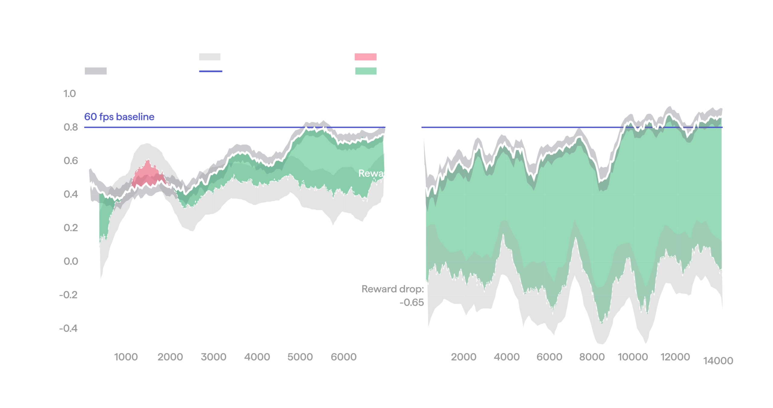
Speed curriculum: a stepwise change in FPS causes a drop in quality that RL later recovers from.
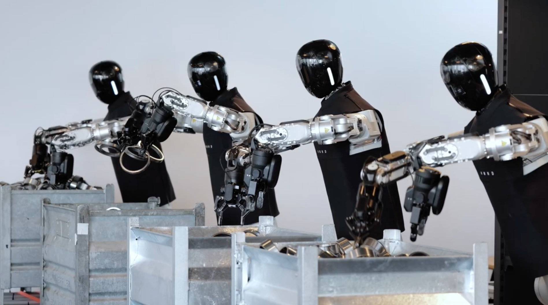
Results
We now show what Gyre delivers on three production tasks from our portfolio, all run on our bimanual Alpha system. The first task is machine feeding, an industrial task where throughput is the main target. The second is object picking and handover, a service task where reliability matters most. The third is bimanual tote handling, another industrial task that requires coordinated bimanual manipulation. In all three cases we start from behavior cloning baselines trained on teleoperation data. Through RL, we achieve improvements in speed and reliability that would be difficult or impossible to teach through demonstration.
Machine feeding
In the machine feeding task, the robot picks bearing rings from a cluttered bin and transfers them to a conveyor table. For this task, we track the following metrics:
- Throughput — transferred rings per hour, the main metric to optimize;
- Pick attempt success rate — a grasp-quality metric; failed grasps trigger retries, which hurt throughput;
- Cycle duration — average time to pick the rings, transfer them, and return to the start. It is not simply the inverse of throughput, because a single cycle can move more than one ring;
- Interventions — how often the system reaches a state it cannot recover from on its own and an operator has to step in. Our policies are generally trained to recover, so we saw no such cases during evals and don’t report this metric.
We start from a behavior cloning baseline that reaches about 291 rings per hour on challenging 110 mm rings at 60 FPS, with a 0.60 pick success rate and a 27.2-second cycle. Pushing the FPS higher on its own only hurts throughput: the policy starts to misgrasp and retry. The goal of RL here is to make the policy robust at the higher speed, so the added FPS turns into throughput rather than failed grasps.
The task consists of two stages, picking rings from the bin and transferring them to the conveyor, both executed end to end by the same BC policy. Picking from clutter is the hard part; transfer is easy. So we apply RL only to the picking stage, which admits an automated reward.
The run took about five days of continuous operation on the hardware. Across it we followed a speed curriculum, starting at 60 FPS and stepping up to 75 and then 90. Each step raised the regrasp rate at first, because the arm starts retracting before the grasp has closed: the gripper cannot close fast enough to keep up at the higher speed. RL then recovered grasp reliability at the new speed before we stepped up again.
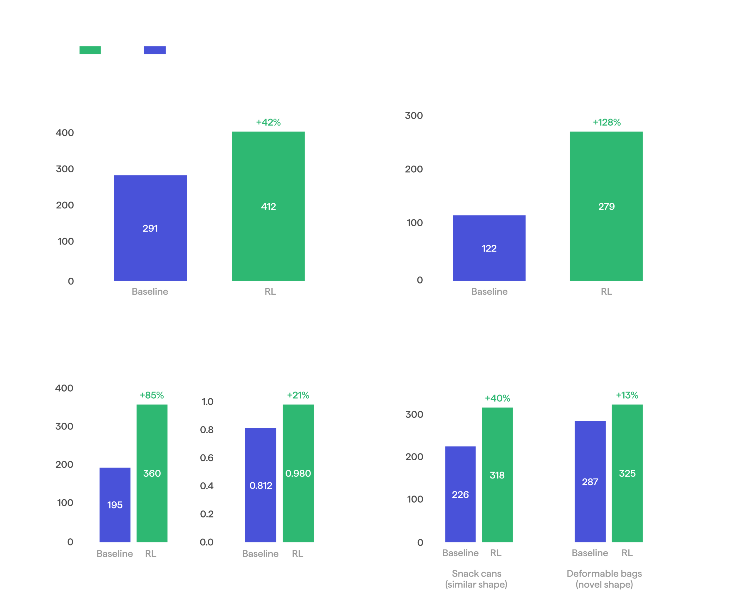
By the end, the RL policy reached 412 rings per hour, a 42% gain over the baseline’s 291. It comes from a shorter cycle (27.2 seconds down to 19.5, since the higher FPS makes every motion faster), and a better pick success rate (0.60 to 0.67), so less time is lost to retries. The confidence interval on cycle time also tightened, so the gain is due to fewer slow outliers in addition to a faster average.
This whole-task gain came from training RL on the picking stage alone. Transfer was never trained with RL, yet the policy still runs the full task end to end, transfer included, at the higher speed the curriculum settled on. This finding means that a behavior does not have to be improved end to end. We can train only the part that actually limits throughput, usually the hardest one, and leave the rest of the policy alone. When robot time is a scarce resource (e.g. during pre-deployment post-training), spending it only on the bottleneck makes the method much more practical.
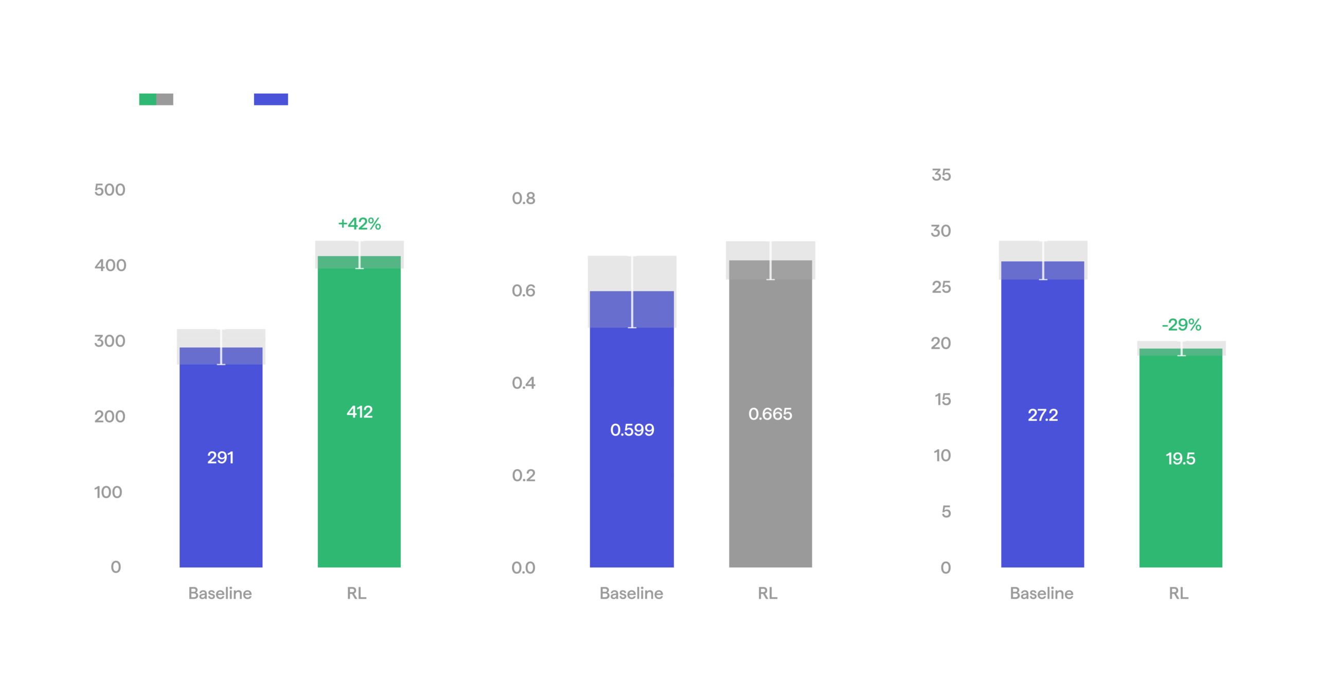
RL vs baseline on machine feeding task.
Machine feeding: Baseline vs RL
Object picking
Our second task is a service application: the robot grasps an item from a cluttered tote and hands it directly to a person standing in front of it, as it might when assisting a customer in a store. The episode ends once the person takes the item.
For this task, we track the following metrics:
- Throughput — successful picks per hour;
- Success rate — the fraction of episodes that end in a successful handover. Failures come in two kinds: a time-out (we use a 30-second limit in our evals) and a false positive, where the robot reports a pick it did not actually make;
- Pick attempt success rate — as in machine feeding, how often a grasp attempt succeeds. Multiple subsequent regrasps can lead to a failure due to a timeout;
- Duration — episode length, regardless of outcome.
The RL run started from a baseline policy that was trained on teleoperation data covering various objects, including those we evaluate on. During RL, by contrast, the model practiced only on bottles of water. We kept the run going for about three days of robot time.
On the bottles, the object RL trained on, every tracked metric improved: throughput rose 85%, mean episode duration fell 35%, and success rate climbed from 80% to 98%. That is a tenfold drop in failures, and a real step toward the 99.9% reliability deployment demands.
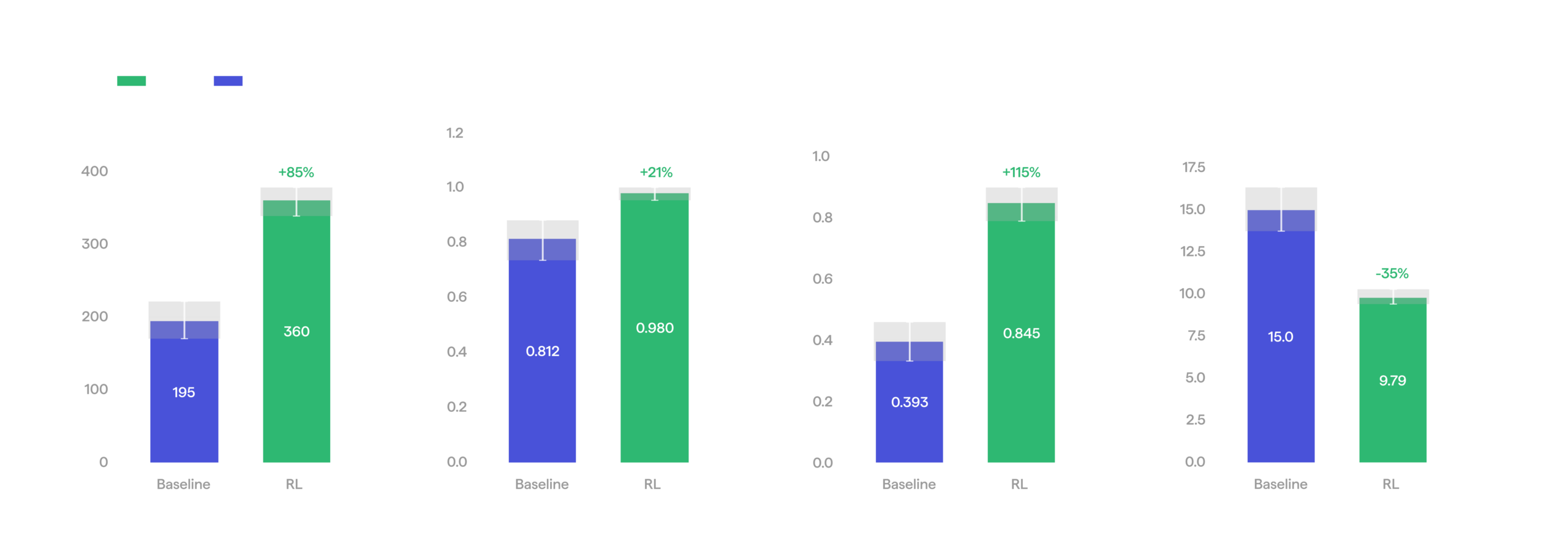
RL vs baseline on bottle picking task.
Bottle picking: Baseline vs RL
We then evaluated the policy on objects it never saw during RL training: cylindrical snack cans, which share some shape similarities with bottles, and small deformable bags. On the cans, RL still improved throughput by 40%: it generalized to a shape it was never rewarded on. On the bags, which have a very different and deformable shape, the gain was a more modest 13%. This was partly because the baseline already performed strongly, and partly because successful bag grasping requires a strategy RL never had a chance to practice. Taken together, these evaluations yield another consequential finding: training on a single object does not overfit the policy to that object; it improves the general skill of picking. This also makes our RL approach more practical: we can train on a subset of objects we care about and still gain on the ones we leave out.
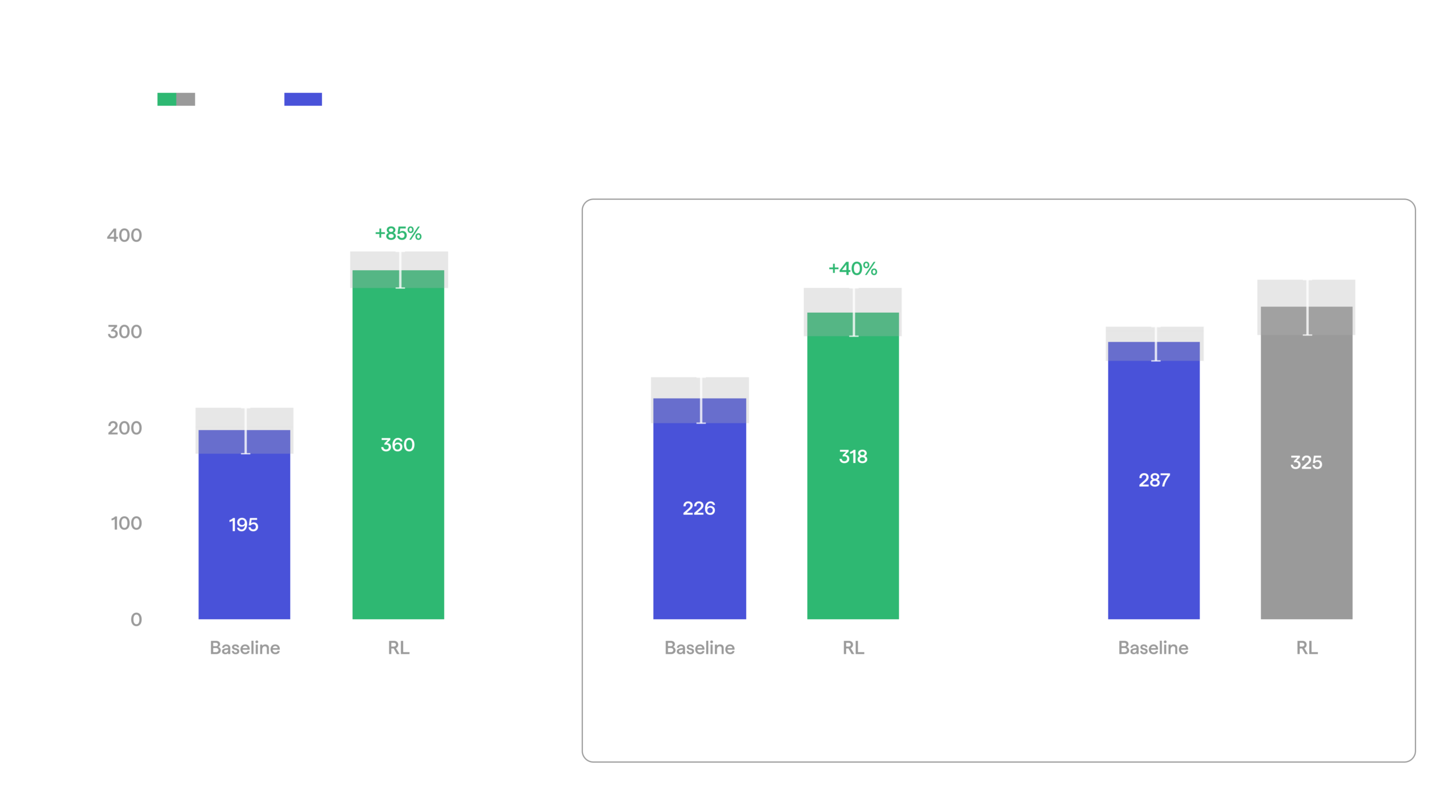
RL brings improvements on objects not seen uring RL training.
Snack can (unseen during RL) picking: Baseline vs RL
We also checked whether the same holds for a capability not practiced during RL training, not just an unseen object. The baseline policy can be told which arm to pick with, left or right. RL did not practice arm conditioning at all, yet it survived intact: when prompted with a specific arm, the RL policy fully complied even when the tote had been placed next to the arm the policy was told not to use. This mirrors what we saw in machine feeding, where training RL on the pick left the transfer stage untouched.
Tote handling
Our third task is bimanual tote handling. Moving totes is one of the most common operations in warehouses and on production lines, where they travel constantly between tables, conveyors, and shelves. In our setup, a tote sits on a table in an arbitrary orientation, and the robot grasps it with both arms and lifts it to chest height, ready to be carried and set down elsewhere. Lifting a tote this way needs both arms acting on the same object at once, a coordination neither earlier task required.
We applied the same stack and the same training recipe with no task-specific changes: the PPO-on-CFM objective, the sparse success reward, the same hyperparameters, and the same speed curriculum we used on machine feeding. The run started from a behavior-cloning baseline and took about four days of robot time. We track throughput, success rate, and episode duration, as before.
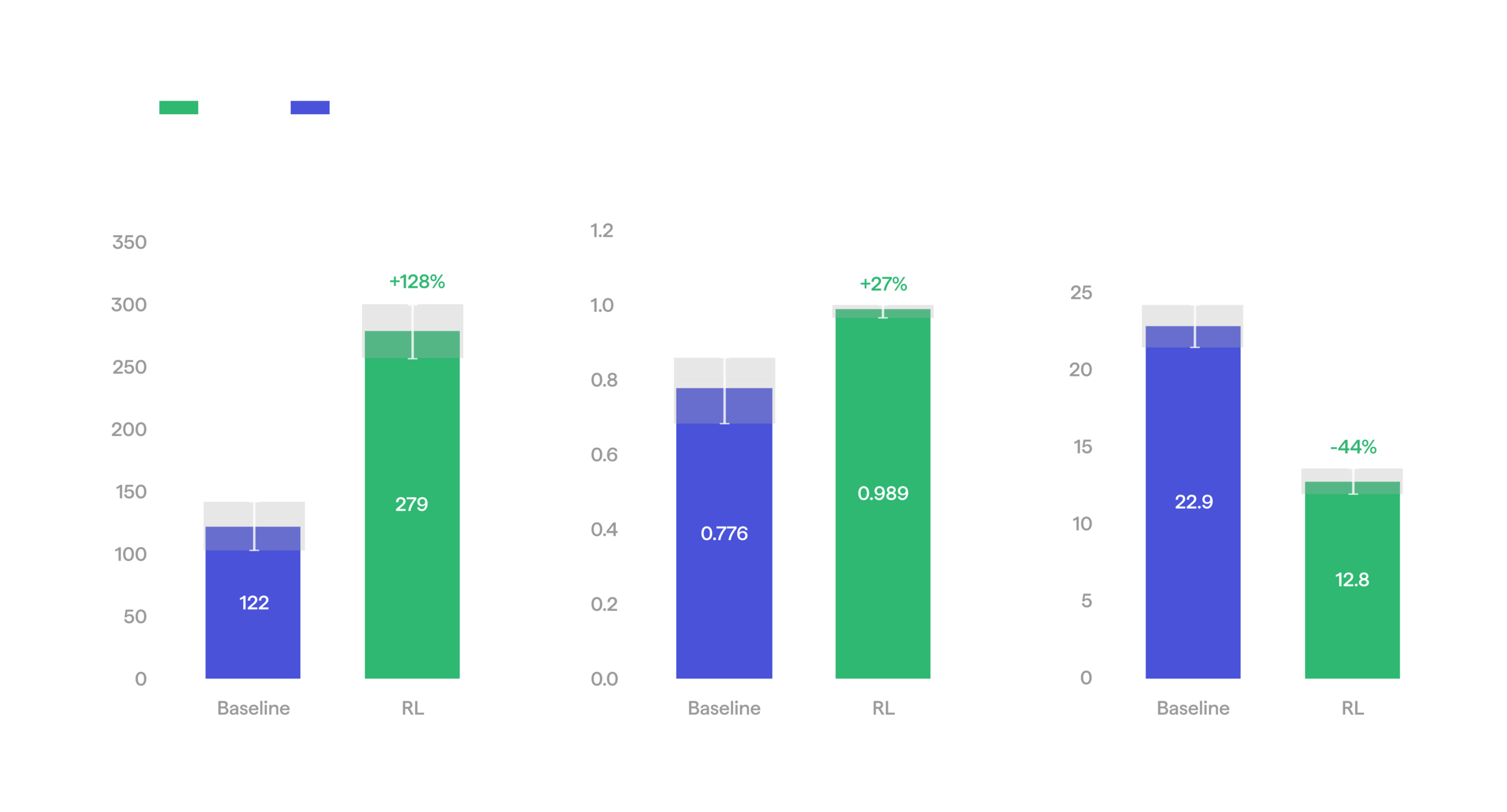
RL vs baseline on tote handling task.
After applying RL, throughput more than doubled, from 122 to 279 totes per hour. Mean episode duration fell 44%, from 22.9 to 12.8 seconds. Success rate climbed from 77.6% to 98.9%, a roughly twentyfold drop in failures, again within sight of the 99.9% bar.
Tote handling: Baseline vs RL
This task differs substantially from the first two, and the method handled it out of the box, with no changes. That gives us confidence that Gyre is general, applicable across the wide range of tasks industrial deployment demands, and can accelerate our product roadmap by turning new capabilities into deployable behaviors much faster.
Discussion
This post laid out why manipulation needs RL, the problems that surface when you run it on modern VLAs, and the stack we built to solve them. On machine feeding, a straightforward application of our method raised throughput by 42% and pushed the policy to 1.5x the speed of its demonstrations. On object picking, RL cut failures tenfold, lifting success from 80% to 98%, within sight of the 99.9% bar. On bimanual tote handling, a very different task, the same method worked with no changes at all, more than doubling throughput and cutting failures roughly twentyfold. RL also did not need end-to-end treatment: training the picking stage alone lifted whole-task throughput, and training on a single object improved picking on objects the policy never saw. To our knowledge, no one has shown end-to-end, vision-based RL on production VLAs on real bimanual humanoid hardware before.
Our findings have also reshaped how we think about the VLA training pipeline.
The role of behavior cloning changes. With RL in the loop, BC no longer has to produce a deployment-ready policy. BC only needs to cover the right behavior modes. RL suppresses what does not work and amplifies and refines what does.
The fleet keeps learning after it ships. A deployed fleet runs the same disaggregated RL loop we run today, and improves itself in the field. The reward signal is already present in the operational model: when a supervisor steps in to correct or rescue a robot, that intervention marks a failure the policy should learn to avoid. Treating interventions as reward turns routine operation into a continuous training signal, so the robots get better at the exact tasks, sites, and conditions they are deployed into. At that point data collection stops being a separate activity: every deployed robot is also a rollout worker, and training throughput grows with the size of the fleet.
RL as a data engine. Every rollout is stored. The collected data enters the pretraining mixture for the next generation of models, and because it is collected on real robots, it carries zero embodiment gap: it comes from exactly the hardware and dynamics the next model will run on. This loop compounds: a policy improved by RL collects better data, better data trains stronger base models, and stronger base models make the next RL run faster and cheaper.
Sample efficiency is our main focus. Our approach is already efficient enough to be practical on hardware, days of robot time per task, but every gain means faster iteration and more tasks per robot-month. We expect the next gains to come from two directions: better RL methods, and getting more out of simulation without paying the full sim-to-real cost, for instance by co-training in sim and on hardware at the same time.
Running RL 24/7 is a proxy for deployment. Our hardware is approaching its production-intent version, and running RL around the clock puts it under deployment-like load long before a customer does. It surfaces the remaining design and operational problems, in hardware and in software, while they are still cheap to fix. It forces the systematic tooling and discipline that reward hacking, environment setup, and the long tail of practical failures demand. This makes Humanoid’s aggressive go-to-market timeline realistic: by the time we deploy, the stack has already run as if deployed.
At Humanoid, we are building a capability factory: a toolset that lets us bootstrap the behaviors we need and polish each one until it meets deployment robustness and KPI targets. Gyre was the missing piece. With it we can take a behavior from working in a demo to robust enough to deploy, and then keep improving it on the fleet that runs it.
Our capability factory already works. What remains is scale: building it out until it powers real automation across the fleet is a large open effort. If you want to build it with us, we are hiring: come work on our RL or simulation stack.
References
Bergmeister, A., Jegelka, S., Nüsken, N., Domingo-Enrich, C., Pidstrigach, J. "Reinforce Adjoint Matching: Scaling RL Post-Training of Diffusion and Flow-Matching Models."
arxiv.orgPhysical Intelligence. "π0.5: a Vision-Language-Action Model with Open-World Generalization."
arxiv.orgBlack, K., Ren, A. Z., Equi, M., Levine, S. "Training-Time Action Conditioning for Efficient Real-Time Chunking."
arxiv.orgZhang, T., et al. "ReinFlow: Fine-tuning Flow Matching Policy with Online Reinforcement Learning."
arxiv.orgHe, H., et al. "Defeating Nondeterminism in LLM Inference." Thinking Machines Lab: Connectionism"
thinkingmachines.aiZhong, T., et al. "Diagnosing Training Inference Mismatch in LLM Reinforcement Learning."
arxiv.orgChen, K., Liu, Z., Zhang, T., et al. "π RL: Online RL Fine-tuning for Flow-based Vision-Language-Action Models."
arxiv.org